GIFSQ ID: FTN-0112
Unit Operations
Unit 1: Introduction to Unit Operations, Units and Material and Energy Balances
Note
Unit 1: Introduction to Unit Operations, Units and Material and Energy Balances
A milk pasteurizer takes in cold raw milk and sends out safe pasteurized milk. Inside the plant, milk is pumped, heated, held, cooled and packed. Each of those steps is a separate job, and each job follows the same few rules of physics. The milk that goes in must come out somewhere: as product, as waste, or held up in the plant. The heat that goes in must come out somewhere too. This unit is about those few rules, the steps they apply to, and the arithmetic that keeps a food factory honest.
Questions to think about
- What is a unit operation, and why does breaking a food process into steps make it easier to study?
- What goes into a unit operation, and what must come out?
- How does a flow chart turn a whole factory into a drawing you can read?
- Why do engineers insist on one system of units, and what goes wrong when units are mixed?
- What is a basis, and why must every material balance state one?
- How do you check whether a heat balance is right, and what do you do when it does not balance?
1.1 What a unit operation is
A food factory looks bewildering from the outside. Milk, fruit, grain, meat and vegetables go in; cartons, cans, jars and bags come out. The processes seem endless and different from each other. The idea of the unit operation cuts through that variety. A unit operation is one basic physical step in a process, a step that cannot usefully be divided into smaller steps. Pumping, heating, cooling, drying, filtering, mixing and grinding are unit operations. A whole process is a chain of them, joined in a set order.
The term was set down in 1915 by Professor Little of the Massachusetts Institute of Technology. His point was simple: every chemical process, at any scale, can be broken into an ordered series of unit operations such as pulverization, drying, crystallization, filtration, evaporation and distillation. The number of these operations is not very large, and generally only a few of them take place in any one process. That insight changed how engineers learn their trade. Instead of studying every factory separately, they study the operations that factories share.
Gould gives the plant view of the same idea. His book lists the operations that matter in fruit and vegetable plants: receiving, materials handling, cleaning wet and dry, quality separation, peeling, disintegration with little change in form such as husking, pitting, coring, shelling and snipping, disintegration with considerable change in form such as cutting, shredding, crushing, comminuting, homogenizing, sheeting and extracting or juicing, separating by screening, floating, settling, filtering and deaeration, concentration, blanching, pumping, mixing and blending, exhausting and vacuuming, salting, seasoning, enrobing, batter and breading, filling, sealing and closure, packaging including coding, extrusion, and preservation by canning, freezing, drying and frying. The list is long, but each item on it is one operation, and each one can be studied on its own.
Ibarz gives the engineering definition. A process is the set of activities or industrial operations that modify the properties of raw materials with the purpose of obtaining products to satisfy the needs of a society. Food process engineering is the science of conceiving, calculating, designing, building and running the facilities where the transformation of agricultural products is carried out at industrial level and as economically as possible. The food engineer should know the basic principles of process engineering, be able to develop new production techniques, and be capable of designing the equipment for a given process.
Food is processed for plain reasons, and Gould lists ten of them: to prevent spoilage, to eliminate waste, to preserve quality, to preserve the nutritive values in the raw materials, to make seasonal fruits and vegetables available year round, to put food in convenient form for the user, to build in chef services, to develop new products such as cucumbers to pickles, tomatoes to catsup, cabbage to kraut, oats to breakfast cereal, corn and potatoes to chips, to put food safely away for emergencies, and to increase the value of the product. Every unit operation in this subject serves one or more of those reasons.
Quick check
Why is it easier to study unit operations than to study each food factory separately?
Check your answer
Because the same few operations appear in many different factories and processes, so learning one operation teaches you something that applies in many places.
1.2 The box: what goes in must come out
Earle draws the whole subject in one picture. A unit operation is a box. Into the box go raw materials and energy. Out of the box come the desired products, the undesired products and energy. The equipment inside the box makes the required changes with as little waste of materials and energy as possible. The desired products are to be maximized and the undesired products minimized. Control over the process is exercised by controlling the flow of energy, or of materials, or of both.
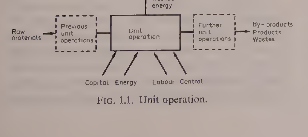
Figure 1.1: Unit operation. The box takes in raw materials and energy and gives out products, by-products, wastes and wasted energy. Capital, energy, labour and control are fed in from below. Reproduced from Earle, Fig. 1.1, p. 3.
The box picture is not a decoration. It is the shape of every balance in this unit. A pasteurizer is a box. A dryer is a box. A whole factory is a row of boxes. When you draw the box, you must name everything that crosses its edge, in and out. Anything you forget to name will show up later as a balance that does not balance.
Two laws govern the box. The law of conservation of mass says that mass is neither created nor destroyed in a physical step: what goes in must come out or stay inside. The law of conservation of energy says the same for energy. Earle puts it in plain words for a milk pasteurizer. The heat energy leaving in the milk must equal the heat energy in the milk entering the pasteurizer, plus the heat energy added by the pump and by the heating water in the heat exchanger, minus the heat energy taken out in the cooling section and the heat energy lost to the surroundings. The same law can be applied to part of a process. In the heating section alone, the heat lost by the heating water must equal the heat gained by the milk plus the heat lost from the heat exchanger to its surroundings.
From these two laws, a balance sheet for materials and for energy can be drawn up at all times for a unit operation. These are called material balances and energy balances, and they are the working tools of the rest of this unit.
Quick check
A dryer takes in wet casein and natural gas. Name three places the mass and the energy can go.
Check your answer
Mass: out as dried product, out as evaporated water, or held up in the dryer. Energy: out in the product and the exhaust, out as heat lost to the surroundings, or stored in the equipment.
1.3 The balance box in full: mass and energy together
Earle's second figure draws the balance box with every stream named. On the left, two streams enter: raw materials, written m_R1, m_R2, m_R3, and energy in the forms of heat, work, chemical and electrical energy, written E_R1, E_R2, E_R3. Inside the box, two things are stored: stored materials m_S1, m_S2, m_S3, and stored energy E_S1, E_S2, E_S3. On the right, five streams leave: products out m_P1, m_P2, m_P3, waste products W1, W2, W3, energy in products E_P1, E_P2, E_P3, energy in wastes E_W1, E_W2, E_W3, and energy losses to surroundings E_L1, E_L2, E_L3.
Mass and energy balance round a unit operation
mR1, mR2, mR3
Heat, Work,
Chemical, Electrical
ER1, ER2, ER3
operation
Stored materials
mS1, mS2, mS3
Stored energy
ES1, ES2, ES3
Figure 1.2: Mass and energy balance. Every stream that crosses the edge of the box is named, with its symbol. Reproduced from Earle, Fig. 2.1, p. 10.
Written as equations, the two laws are:
Mass in = Mass out + Mass stored
Raw Materials = Products + Wastes + Stored Materials
Energy in = Energy out + Energy stored
The sums are written with the Greek letter sigma, which means the sum of all terms. So the total raw materials are the sum of m_R1, m_R2, m_R3, and the same for products, wastes and stored materials. The energy balance is the sum of the energy entering, the energy leaving with products, the energy leaving with waste materials, the energy lost to surroundings, and the energy stored.
The same law applies to each component separately, as long as no chemical change is taking place. In a sugar plant, if the total sugar going in is not equalled by the purified sugar plus the sugar in the waste liquors, then something is wrong. Sugar is either being burned, which is a chemical change, or accumulating in the plant, or going unnoticed down the drain. In that case the balance gains a term for the unknown loss, and the balance reads: Raw Materials = Products + Waste Products + Stored Products + Losses. That unknown loss is a real thing to go and find, not a number to hide.
Quick check
A balance on sugar does not add up: less sugar comes out than went in, and nothing is stored. Name two things that could have happened.
Check your answer
The sugar could have been changed chemically, for example burned or browned, or it could be leaving unnoticed, for example down a drain.
1.4 Reading a flow chart: olive oil and a canning line
Food processes are usually drawn as flow charts. Ibarz explains the most common kind: each stage of the process is a block or rectangle, the name of the stage is written inside the rectangle, and arrows join the blocks to show the way the materials flow. Other kinds of flow chart show the equipment or the instruments, but the block chart is the one to learn first.
The olive oil chart in Ibarz is a good first chart to read, because it shows a split. Olives go into WASHING, then PRESSING. From pressing, the stream splits in two. One branch is the oil from the press, which goes to CENTRIFUGATION and comes out as virgin oil. The other branch is the bagasse, the pressed olive pulp, which goes to DRYING and then to EXTRACTION, and comes out as bagasse oil, with exhausted bagasse leaving the extraction step.
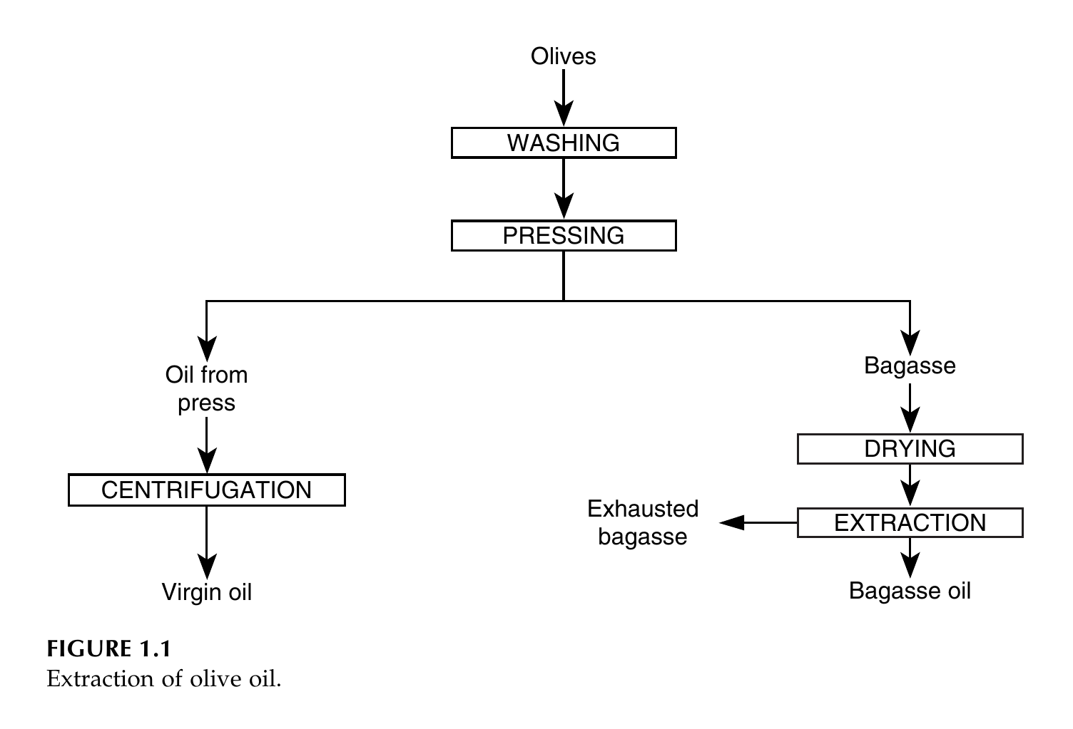
Figure 1.3: Extraction of olive oil. Pressing gives three outputs: virgin oil from centrifugation of the pressed oil, bagasse oil from extraction of the dried bagasse, and exhausted bagasse leaving the extraction step. Reproduced from Ibarz, Fig. 1.1, p. 3.
Two more Ibarz charts show the same idea in other foods. Fruit juice goes Fruit, CRUSHING, PRESSING with pulp leaving, Juice 12 degrees Brix, PRE-CONCENTRATION with water and aromas leaving, Juice 15 degrees Brix, ENZYMATIC TREATMENT, CLARIFICATION, EVAPORATION with water leaving, Juice 70 degrees Brix, COOLING, STORAGE. Soluble coffee goes roasted coffee, GRINDING, EXTRACTION with hot water in and solid waste out, coffee exhaust as a diluted solution, EVAPORATION with water vapour out, coffee extract as a concentrated solution, DRYING with water out, soluble coffee. In each chart, the side streams matter as much as the main line: the pulp, the water, the aromas and the solid waste are all named, because a balance must account for them.
Gould's canning chart is a whole factory on one page. It runs from top to bottom: Harvest, Receiving, Washing, Peeling, Husking, Pitting, Coring, Etc., Separating, Grading, Sorting For Size, Color, Solids and Defective Removal, Holding By Quality, Pumping, Blanching, Dewatering, Filling, Exhausting, Container Closing, Cooker, Cooler, Labeler, Casing, To Warehouse. The original draws each step inside a pictogram shaped like the equipment used for that step. The list below keeps the same steps, in the same order, with the same words, in plain boxes.
Generic Fruit and Vegetable Canning Flow Chart
↓
↓
↓
↓
↓
↓
↓
↓
↓
↓
↓
↓
↓
↓
Figure 1.4: Generic Fruit and Vegetable Canning Flow Chart. Steps, order and wording are as in the book. The original draws each step inside an equipment pictogram; the shapes are simplified here to labelled boxes, and the pictogram shapes are listed as a diagram flag in DIAGRAM-FLAGS.md. Reproduced from Gould, Fig. 1.1, p. 4.
Notice what the canning chart does not show: no quantities, no temperatures, no times. A flow chart shows the order of steps and the direction of flow. The numbers come later, in the balances. That is why the two tools belong together: the chart says what happens in what order, and the balance says how much.
🤔 Pause and think: pick a food you know well, such as bread, jam or yoghurt. Sketch its steps as boxes with arrows, in order. Where does the stream split into two, as in the olive oil chart? What leaves as a side stream, and where does it go?
1.5 The families of unit operations
When you look at many flow charts, the same stages keep appearing. Ibarz groups them by the property that is transferred. A body can change in its mass, its energy or its velocity, so unit operations fall into mass transfer, heat transfer and momentum transfer, plus operations where heat and mass move together, plus a few that fit none of those groups.
Momentum transfer operations are about two phases at different velocities in contact. They divide into three groups: internal circulation of fluids, which is the movement of fluids through the inside of tubing, including pumps, compressors, blowers and fans, and the instruments that measure fluid properties such as diaphragms, venturi meters and rotameters; external circulation of fluids, where the fluid moves round the outside of a solid, including flow through porous fixed beds, fluidized beds and pneumatic transport; and solids movement within fluids, which is the basis for separating solids in a fluid, including sedimentation, filtration and ultrafiltration.
Mass transfer operations are controlled by the diffusion of a component within a mixture: distillation, which separates components by taking advantage of vapour pressure differences; absorption, where a component of a gas mixture is absorbed by a liquid according to its solubility, with desorption as the opposite process; extraction, based on dissolving a mixture in a selective solvent, liquid to liquid or solid to liquid, the last also called washing or lixiviation; adsorption, also called sorption, where components of a fluid are removed by retention on the surface of a solid; and ionic exchange, the substitution of ions of a solution with another exchange agent.
Heat transfer operations are controlled by temperature gradients: conduction, where heat flows in the direction of temperature decrease in a continuous material medium with no large scale movement of mass; convection, the enthalpy flow that goes with a moving fluid, which can be natural or forced; and radiation, energy transmission by electromagnetic waves, which needs no material medium. Thermal treatments such as sterilization and pasteurization, evaporation, heat exchangers, ovens and solar plates are all studied from these three mechanisms.
Simultaneous mass and heat transfer operations carry a concentration gradient and a temperature gradient at the same time: humidification and dehumidification, including the cooling of a liquid; crystallization, the formation of solid glassy particles within a uniform liquid phase; and dehydration, the removal of a liquid contained in a solid, where heat changes the liquid into vapour, or in freeze drying, where the solid phase is removed by sublimation, changing it into vapour.
Complementary operations fit none of the transport groups: grinding, milling, sieving, mixing of solids and pastes, and similar steps. The physical, chemical and biochemical stages together make up the unit operations of the food industry, and their purpose is the separation of two or more substances present in a mixture, or the exchange of a property due to a gradient.
This subject follows that map. Units 2 and 3 cover momentum and heat transfer. Unit 4 covers thermal processing, refrigeration and freezing. Later units cover mass transfer, drying, evaporation, distillation, extraction, membranes, mechanical separations, size reduction and mixing.
Quick check
A plate heat exchanger heats milk with hot water. Which transfer family does it belong to, and what is the gradient that drives it?
Check your answer
Heat transfer, driven by the temperature gradient between the hot water and the milk.
1.6 Steady and unsteady, batch and continuous
A system is under steady state when all the physical variables remain constant and unchanging along time, at any point of the system, although they may be different from one point to another. When the characteristic intensive variables vary through the system at a given moment, and the variables at each point vary along time, the state is called unsteady. The variables to consider may be mechanical or thermodynamic: volume, velocity and similar quantities on one side, and viscosity, concentration, temperature and pressure on the other.
The same distinction shapes how a factory runs. In a discontinuous operation, also called batch or intermittent, the raw material is loaded into the equipment, the conditions for transformation are prepared, the transformation is carried out, the products are unloaded, and the equipment is cleaned. The steps are: loading, preparation, transformation, unloading, cleaning. The batch operation takes place under unsteady state, since its intensive properties vary along time. Crushing oily seeds to obtain oil is a batch example in the book.
In a continuous operation, loading, transformation and unloading happen at the same time. Cleaning is carried out at set intervals, and production must stop for it. Continuous operations take place under steady state: the characteristic intensive variables may vary at each point of the system but do not vary along time. Reaching an absolute steady state is hard, since there may be unavoidable fluctuations. Rectification of an alcohol and water mixture is the book's continuous example.
A semicontinuous operation sits between the two. Some materials are loaded and stay in the equipment for a set time in a discontinuous way, while other materials enter or leave continuously, and the accumulated materials must be unloaded after a time. In solvent extraction of oil, flour is loaded and the solvent is fed continuously; after some time the flour has run out of oil and must be replaced.
Continuous operation has advantages: the loading and unloading stages are removed, automation is possible so the work force is reduced, the composition of products is more uniform, and thermal energy is better used. It has disadvantages too: raw materials should have a uniform composition to avoid fluctuations, starting is usually expensive so stops should be avoided, changes in product demand need large stocks of raw materials and products, and the automated equipment is more expensive and delicate. Continuous operation is unsteady during starts and stops, but once running well it may be treated as steady state. When low production is needed, discontinuous working is recommended; when high production is needed, continuous working is more profitable.
For balances, the distinction matters in one practical way. In a continuous process, time enters the balance and the balance is written per unit time, such as per hour. In a batch process, the balance is written for the whole batch. Either way, if there is no accumulation, what goes in must come out over the chosen time interval.
Quick check
A jam kettle is filled, heated, emptied and cleaned, then filled again. Is that batch or continuous, and is it steady or unsteady?
Check your answer
Batch, and unsteady, because the temperature and the contents change with time through the cycle.
1.7 Dimensions and units
All engineering deals with definite and measured quantities, so it depends on making measurements. A measurement compares the unknown with the known: weighing a material compares it with a standard weight of one kilogram. The record of a measurement has three parts: the dimension of the quantity, the unit which represents a known or standard quantity, and a number which is the ratio of the measured quantity to the standard. A rod 1.18 m long gives a dimension, length, a standard unit, the metre, and a number 1.18, the ratio of the length of the rod to the standard length of 1 m.
Everyday engineering quantities can all be expressed in terms of a small number of dimensions: length, mass, time and temperature. For convenience, force is added as another dimension, because it simplifies many calculations even though force can be expressed in terms of the others. Dimensions are written in square brackets: length [L], mass [M], time [θ], temperature [T] and force [F]. The Greek letter theta is used for time because time and temperature both begin with the letter t in English.
From those five, everything else follows. Area is [L]², volume is [L]³, velocity is [L][θ]⁻¹, acceleration is [L][θ]⁻², pressure is force per unit area [F][L]⁻², density is mass per unit volume [M][L]⁻³, energy is force times length [F][L], and power is energy per unit time [F][L][θ]⁻¹. In heat transfer, the heat transfer coefficient h is the quantity of heat energy transferred through unit area, in unit time, with unit temperature difference, so its dimensions are [F][L]⁻¹[θ]⁻¹[T]⁻¹ in the book's notation, or in mass terms [M][θ]⁻³[T]⁻¹.
Units are the standards in which dimensions are measured. In the SI system, the metre is defined in terms of the wavelength of light, the standard kilogram is the mass of a standard lump of platinum and iridium, the second is the time taken for light of a given wavelength to vibrate a given number of times, and the degree Celsius is one hundredth part of the temperature interval between the freezing point and the boiling point of water at standard pressure. The unit of force, the newton, is the force which gives an acceleration of 1 m s⁻² to a mass of 1 kg. The energy unit, the newton metre, is called the joule, and the power unit, 1 J s⁻¹, is called the watt.
Ibarz gives the same system in a table, with the dimensions in mass, length and time form. The fundamental and derived units of the International System are:
Table 1.1: International Unit System (Ibarz Table 2.5)
| Magnitude | Unit | Abbreviation | Dimension |
|---|---|---|---|
| Length | metre | m | L |
| Mass | kilogram | kg | M |
| Time | second | s | T |
| Force | Newton | N | MLT⁻² |
| Energy | Joule | J | ML²T⁻² |
| Power | Watt | W | ML²T⁻³ |
| Pressure | Pascal | Pa | ML⁻¹T⁻² |
| Frequency | Hertz | Hz | T⁻¹ |
Table 1.1: International Unit System, Ibarz Table 2.5, p. 35.
Ibarz also explains the older systems. Absolute unit systems take mass as the third fundamental magnitude: the c.g.s., the Giorgi (MKS) and the English (FPS) systems. Technical unit systems take force as fundamental. Engineering unit systems take length, time, mass and force all as fundamental. When mass and force are both taken as fundamental, a correction factor gc must be inserted, because the two are related by the basic principle of dynamics: gc times force equals mass times acceleration. In the metric engineering system gc is 9.81 kg m per kg force s², and in the English system it is 32.17 lb ft per lb force s². The International System was adopted from the MKS system to unify the use of unit systems, and many engineering journals and books are now edited only in SI.
When a unit is too big or too small, prefixes give multiples and submultiples, generally as powers of 10³: tera 10¹², giga 10⁹, mega 10⁶, kilo 10³, hecto 10², deca 10¹, deci 10⁻¹, centi 10⁻², milli 10⁻³, micro 10⁻⁶, nano 10⁻⁹, pico 10⁻¹², femto 10⁻¹⁵, atto 10⁻¹⁸. Time is the exception: its multiples are not decimalized, so minutes, hours and days still sit beside micro and milli seconds, and care must be taken to use the right multiplying factors.
Practical note: never write a number in a food factory without its unit. A temperature of 121 with no unit could be Celsius or Fahrenheit, and the difference between those two is the difference between a safe can and a spoiled one. A flow of 12.4 with no unit could be cubic feet per hour or cubic metres per hour, and the two differ by a factor of 35.
1.8 Dimensional consistency and conversion factors
All physical equations must be dimensionally consistent: both sides of the equation must reduce to the same dimensions. Dimensions can be handled algebraically, divided, multiplied or cancelled. That test is sometimes useful as an aid to memory. If an equation is written down and on checking is not dimensionally homogeneous, then something has been forgotten.
Earle's first worked example shows the test. A particle travels at a uniform velocity for a time θ, and the distance travelled is L = vθ. Length has dimensions [L] and time has dimensions [θ], so the dimensions of velocity must be [L][θ]⁻¹. That is the whole check, and it is worth doing before any arithmetic.
Unit consistency is the companion rule: the units used for the dimensions should be chosen from a consistent group, in this book the SI system. Very often quantities are measured in mixed units, and then all the times, or all the lengths, must be put into one unit before calculating. Where tabulated data are only available in non standard units, conversion tables such as those in Earle's Appendix 2 have to be used.
The conversion factor method is the safe way to do it. A conversion factor is a fraction whose numerator and denominator are equal, so multiplying by it changes the units but not the value. To convert 10 grams into pounds, the book uses 1 lb = 0.4536 kg and 1000 g = 1 kg: 10 g times (1 lb / 0.4536 kg) times (1 kg / 1000 g) = 2.2 x 10⁻² lb. Units cancel in the same way as numbers.
Worked example: milk flowing through a pipe (Earle Example 1.3)
Milk is flowing through a full pipe whose diameter is 1.8 cm. The only measure available is a tank calibrated in cubic feet, and it takes 1 hour to fill 12.4 ft³. What is the velocity of flow in the pipe?
Velocity is [L][θ]⁻¹, so in SI the units are m s⁻¹. Volume flow is 12.4 ft³ per hour. From Appendix 2, 1 ft³ = 0.0283 m³, so the volume flow is 12.4 x 0.0283 / 3600 = 9.75 x 10⁻⁵ m³ s⁻¹. The area of the pipe is πD²/4 = π(0.018)²/4 = 2.54 x 10⁻⁴ m². Velocity is volume flow divided by area: 9.75 x 10⁻⁵ / 2.54 x 10⁻⁴ = 0.38 m s⁻¹.
Diagram: Milk flowing through a pipe (Earle Example 1.3)
Tank: 12.4 ft³ filled in 1 hour
↓
Area 2.54 x 10⁻⁴ m²
↓
Volume flow 9.75 x 10⁻⁵ m³ s⁻¹
Velocity 0.38 m s⁻¹
Diagram for Earle Example 1.3: the tank measures the volume flow, the pipe fixes the velocity.
Worked example: thermal conductivity of aluminium (Earle Example 1.5)
The thermal conductivity of aluminium is given as 120 Btu ft⁻¹ h⁻¹ °F⁻¹. Convert it to J m⁻¹ s⁻¹ °C⁻¹. From Appendix 2, 1 Btu = 1055 J, 0.3048 m = 1 ft, 1 h = 3600 s, and 1 °F = (5/9) °C. Multiplying through: 120 x 1055 / 0.3048 / 3600 x (5/9) = 208 J m⁻¹ s⁻¹ °C⁻¹. The same method works for any conversion, however complicated, if it is applied systematically.
No diagram: this example is a pure unit conversion, with no equipment, stream or setup to draw.
One loose mode of expression causes confusion, and Earle warns against it. Acceleration due to gravity is often written as 9.81 metres per second per second, which looks like m/s/s, that is m s⁻² written badly. A better way is g = 9.81 m/s², which is clearly the same as 9.81 m s⁻². Precision in writing down units is a great help in solving problems.
Quick check
An equation gives a heat flow in J s⁻¹ on the left and in kg m² s⁻³ on the right. Is it dimensionally consistent?
Check your answer
Yes. A joule is a newton metre, which is kg m² s⁻², so J s⁻¹ is kg m² s⁻³. Both sides match.
1.9 Dimensionless numbers: a sense of proportion
It is often easier to see a quantity if it is expressed as a ratio, and ratios have the great advantage of being dimensionless. If a car is going at twice the speed limit, that dimensionless ratio draws attention to the speed at once. These ratios are often used in process engineering, comparing the unknown with some well known material or factor.
Specific gravity is the simplest example. It is the ratio of the weight of a volume of a substance to the weight of an equal volume of water. If the density of water is known, the density of the substance follows from density = specific gravity times density of water. Perhaps the most important attribute of a dimensionless ratio is that it gives an immediate sense of proportion. If the specific gravity of a solid is greater than 1, that solid will sink in water. The fact that the specific gravity of iron is 7.88 makes the quantity more easily seen than the equivalent statement that the density of iron is 7880 kg m⁻³. A dimensionless ratio does not depend on the units used, provided the units are consistent for each dimension.
Dimensionless ratios are used all through fluid flow and heat flow. They may look more complicated than specific gravity, but they work the same way, expressing ratios of the unknown to the known. They are then called dimensionless numbers, often named after a person: Reynolds number, Prandtl number and Nusselt number. When evaluating them, all units must be kept consistent, using conversion factors where necessary. The Reynolds number returns in Unit 2, where it decides whether flow in a pipe is smooth or turbulent.
Quick check
A syrup has a specific gravity of 1.3. What is its density, and will it sink in water?
Check your answer
Density is 1.3 times 1000 kg m⁻³, which is 1300 kg m⁻³. Yes, it will sink, because its specific gravity is greater than 1.
1.10 Material balances: choosing a basis
The first step in a material balance is to look at the three basic categories: materials in, materials out and materials stored. Then the materials in each category have to be considered: whether they are to be treated as a whole, a gross mass balance, or whether various constituents should be treated separately, and if so which ones. Dry solids as opposed to total material really means separating the two groups of constituents, non water and water. A fuller dissection can separate out chemical types such as minerals, or chemical elements such as carbon. The choice depends on the reasons for making the balance and on the information required. Expensive raw materials are more likely to be followed than cheaper ones, and products more than waste materials.
Having decided which constituents need consideration, the basis for the calculations has to be decided. It might be some mass of raw material entering in a batch system, or some mass per hour in a continuous process. It could be some mass of a predominant constituent, for example 100 kg of flour entering a bakery, or an unchanging constituent such as the inert nitrogen in combustion calculations, or the carbon added in a fermentation system, or the inert non oil constituents of oilseeds in an oil extraction process. Sometimes it does not matter what basis is chosen, and then a convenient quantity such as the total raw materials into one batch, or passed per hour into a continuous process, is selected. Having selected the basis, the units may be chosen, such as mass, or concentrations by weight or by mole if reactions matter. In this book, percentage means percentage by weight unless otherwise stated, and the term mole means a mass equal to the molecular weight in kilograms.
Concentrations can be expressed in many ways: weight per weight, weight per volume, molar concentration and mole fraction. The weight per weight concentration is the weight of solute divided by the total weight of the solution. The weight per volume concentration is the weight of solute in the total volume of the solution. The molar concentration is the number of molecular weights of the solute, expressed in kg, in 1 m³ of the solution. The mole fraction is the ratio of the number of moles of the solute to the total number of moles of all species present. For gases, concentrations are measured in weight concentrations or as partial pressures, related through the gas law pV = nRT, where R is 0.08206 m³ atm mole⁻¹ K⁻¹.
Every mass balance solution in this unit follows the same four labelled stages, in the order the books work them: (1) draw and label the flow diagram, with every stream that crosses the edge of the box named; (2) state the basis and the constituents to be followed; (3) write the balance equations, one for the total mass and one for each constituent followed; (4) solve and check, so the balance closes. Earle works his balances from the flow diagram in Chapter 2, Ibarz sets out the same order in section 1.8, and Brennan follows it in section 11.4.2. None of the books numbers the stages; the four labels are the working order used here, so every worked example below is laid out in that shape.
Worked example: skim milk from whole milk (Earle Example 2.1)
Skim milk is prepared by removing some fat from whole milk. The skim milk contains 90.5% water, 3.5% protein, 5.1% carbohydrate, 0.1% fat and 0.8% ash. If the original milk contained 4.5% fat, calculate its composition, assuming that fat only was removed and that there are no losses.
Basis: 100 kg of skim milk, which contains 0.1 kg of fat. Let the fat removed be x kg.
Diagram: Removing fat from whole milk (Earle Example 2.1)
In: whole milk (100 + x) kg, 4.5% fat
↓
↓
Out: skim milk 100 kg, 0.1% fat
Out: removed fat x kg
Found value: x = 4.6 kg
Diagram for Earle Example 2.1: fat is removed from whole milk to give skim milk. See Figure 1.2 for the general form of the balance box.
Equations: the total original fat is (x + 0.1) kg and the total original mass is (100 + x) kg. Since the original fat content was 4.5%: (x + 0.1)/(100 + x) = 0.045.
Solve and check: x = 4.6 kg of fat removed. The balance closes: 100 kg of skim milk plus 4.6 kg of removed fat is 104.6 kg of whole milk.
Composition: the whole milk composition is then fat 4.5%, water 86.5%, protein 3.3%, carbohydrate 4.9% and ash 0.76%.
Note: the book prints 0.8% ash for the whole milk. That is a book error: the skim milk ash of 0.8 kg in 104.6 kg of whole milk is 0.76%, so the value 0.76% is kept here.
Worked example: salt solution concentrations (Earle Example 2.2)
A solution of common salt in water is prepared by adding 20 kg of salt to 100 kg of water, to make a liquid of density 1323 kg m⁻³.
Diagram: Making a salt solution (Earle Example 2.2)
In: salt 20 kg
In: water 100 kg
↓
↓
Out: solution 120 kg, density 1323 kg m⁻³
Diagram for Earle Example 2.2: salt and water are mixed to make the solution. This is a setup aid only: the example is about the definitions of concentration, not about solving a balance. See Figure 1.2 for the general form of the balance box.
(a) Weight per weight: the weight fraction of salt is 20/(100 + 20) = 0.167, or 16.7% weight per weight.
(b) Weight per volume: 1 m³ of solution weighs 1323 kg and contains (20/120) x 1323 = 220.5 kg of salt per m³, which is 22.1% weight per volume.
(c) Mole fraction: 0.058, from 0.34 moles of salt against 5.56 moles of water.
(d) Molar concentration: 3.77 moles per litre.
Worked example: carbonation of a soft drink (Earle Example 2.4)
The total quantity of carbon dioxide required is the equivalent of 3 volumes of gas to one volume of water at 0 °C and atmospheric pressure. Take a basis of 1 m³ of water, which is 1000 kg. The volume of carbon dioxide added is 3 m³. From the gas equation pV = nRT, with p = 1 atm, V = 3 m³, R = 0.08206 m³ atm mole⁻¹ K⁻¹ and T = 273 K, the number of moles is n = 0.134 kmol. The molecular weight of carbon dioxide is 44, so the weight added is 0.134 x 44 = 5.9 kg. The mass fraction in the drink is 5.9/(1000 + 5.9) = 5.9 x 10⁻³, and the mole fraction is 0.134/(55.56 + 0.134) = 2.4 x 10⁻³.
Diagram: Carbonation of a soft drink (Earle Example 2.4)
In: water 1 m³ (1000 kg)
In: carbon dioxide 3 m³
↓
↓
Out: carbonated drink 1005.9 kg, containing 5.9 kg of carbon dioxide
Diagram for Earle Example 2.4: water and carbon dioxide are combined in the carbonator. See Figure 1.2 for the general form of the balance box.
Worked example: milk separation in a continuous centrifuge (Earle Example 2.5)
35,000 kg of whole milk containing 4% fat is to be separated in a 6 hour period into skim milk with 0.45% fat and cream with 45% fat. What are the flow rates of the two output streams?
Basis: 1 hour of whole milk flow.
Mass in: whole milk 5833 kg (35,000/6), of which fat is 5833 x 0.04 = 233 kg.
Diagram: Milk separation in a centrifuge (Earle Example 2.5)
In: whole milk 5833 kg h⁻¹, 4% fat
↓
↓
Out: cream x = 465 kg h⁻¹, 45% fat
Out: skim milk 5368 kg h⁻¹, 0.45% fat
Diagram for Earle Example 2.5: whole milk is separated in a centrifuge into cream and skim milk. See Figure 1.2 for the general form of the balance box.
Mass out: cream x kg, with fat 0.45x; skim milk (5833 - x) kg, with fat 0.0045(5833 - x).
Material balance on fat: 233 = 0.0045(5833 - x) + 0.45x.
Solve: x = 465 kg.
Answer: the cream flows at 465 kg h⁻¹ and the skim milk at 5833 - 465 = 5368 kg h⁻¹.
The time unit has to be considered carefully in continuous processes. Usually there are three periods: start up, continuous processing in steady state, and close down. The time interval over which measurements are taken must be long enough to allow for slight periodic or chance variation.
Worked example: blending minced meat (Earle Example 2.7)
A plant is producing minced meat which must contain 15% fat, made from boneless cow beef with 23% fat and boneless bull beef with 5% fat. Let the proportions be A of cow beef to B of bull beef. A balance on fat gives A x 0.23 + B x 0.05 = (A + B) x 0.15, so A(0.08) = B(0.10), and A/(A + B) = 10/18 = 5/9. For 100 kg of product, that is 55.6 kg of cow beef to 44.4 kg of bull beef.
Diagram: Blending minced meat (Earle Example 2.7)
In: cow beef A kg, 23% fat
In: bull beef B kg, 5% fat
↓
↓
Out: minced meat 100 kg, 15% fat
Found values: A = 55.6 kg, B = 44.4 kg
Diagram for Earle Example 2.7: two beefs are blended to a fixed fat content. See Figure 1.2 for the general form of the balance box.
Worked example: potato drying (Earle Example 2.8)
Potatoes are dried from 14% total solids to 93% total solids. What is the product yield from each 1000 kg of raw potatoes, assuming that 8% by weight of the original potatoes are lost in peeling?
Take a basis of 1000 kg of potatoes entering.
Diagram: Potato drying in two stages (Earle Example 2.8)
In: raw potatoes 1000 kg (solids 140 kg, water 860 kg)
↓
↓
Out: peelings 80 kg (solids 11 kg, water 69 kg)
On: 920 kg to the dryer (solids 129 kg, water 791 kg)
↓
↓
Out: evaporated water 781 kg
Out: dried product 139 kg (solids 129 kg, water 10 kg)
Diagram for Earle Example 2.8: potatoes are peeled, then dried in two stages. See Figure 1.2 for the general form of the balance box.
Mass in: potatoes 1000 kg: solids 140 kg, water 860 kg.
Mass out:
| Stream | Solids (kg) | Water (kg) | Total (kg) |
|---|---|---|---|
| Peelings | 11 | 69 | 80 |
| Dried product | 129 | 10 | 139 |
| Evaporated water | - | 781 | 781 |
| Total out | 140 | 860 | 1000 |
The dryer therefore receives 129 kg of solids and 791 kg of water. The dried product at 93% solids weighs 129/0.93 = 139 kg, with 10 kg of associated water. Water evaporated is 781 kg. The total out is 139 kg of product plus 80 kg of peelings plus 781 kg of evaporated water, which is 1000 kg, so the balance closes. The product yield is 139/1000 = 14%.
Quick check
A balance on a drying process shows 1000 kg in and 139 kg of product plus 80 kg of peelings out, but only 700 kg of water evaporated. What is missing?
Check your answer
81 kg of water: 1000 minus 139 minus 80 is 781 kg of water that must have evaporated, not 700 kg. Either a measurement is wrong or water is held up in the dryer.
1.11 Energy balances: heat is the form that matters most
Energy takes many forms: heat, kinetic energy, chemical energy, potential energy. Because of interconversion it is not always easy to isolate separate constituents of energy balances. In many heat balances other forms of energy are insignificant; in some mechanical situations, such as the flow of fluids in pipes, the frictional losses appear as heat but the details of the heating need not be considered. Practical energy balances therefore tend to focus on the dominant aspect. In this book the two applications are heat balances, which are the basis for heat transfer, and the energy balances used in analysing fluid flow.
A heat balance is a useful description of important cost and quality aspects of a food process situation. Enthalpy, total heat, is conserved, and enthalpy balances can be written round items of equipment, process stages or the whole plant, assuming no appreciable heat is converted to other forms of energy such as work. Enthalpy is always referred to some reference level or datum, so the quantities are relative to that datum. Working out energy balances is then a matter of considering the quantities of materials involved, their specific heats, and their changes in temperature or state, since latent heats from phase changes are often met.
Two kinds of heat must be kept apart. Sensible heat is the heat which, when added or subtracted from food materials, changes their temperature and can be sensed. It is calculated by multiplying the mass by the specific heat by the change in temperature, with units of specific heat in J kg⁻¹ °C⁻¹. Latent heat is the heat required to change, at constant temperature, the physical state of materials from solid to liquid, liquid to gas, or solid to gas. Its units are J kg⁻¹, and total latent heat is the mass changing phase multiplied by the latent heat. Heat is absorbed or evolved by some reactions in food processing, but usually the quantities are small compared with sensible and latent heat.
The heat balance can be drawn as a picture, Earle's Fig. 2.2. Heat enters from electricity, from fuel by combustion, from mechanical sources, in raw materials and from the surroundings. Heat leaves in products, in wastes, to the surroundings, or is stored. The balance is: heat in equals heat out plus heat stored.
Worked example: freezing bread (Earle Example 2.10)
It is desired to freeze 10,000 loaves of bread, each weighing 0.75 kg, from an initial room temperature of 18 °C to a final store temperature of -18 °C. The total freezing time is to be 6 hours, and the maximum heat demand is twice the average demand. Estimate the maximum demand.
Three estimates of the enthalpy change are given in the book. Tabulated data give specific heat above freezing 2.93 kJ kg⁻¹ °C⁻¹, below freezing 1.42 kJ kg⁻¹ °C⁻¹, latent heat of freezing 115 kJ kg⁻¹ and freezing temperature -2 °C, giving a total of 196 kJ kg⁻¹. A formula based on 36% water gives 182 kJ kg⁻¹. Enthalpy and temperature data for bread of 36% moisture give a total of 145 kJ kg⁻¹. The differences come from the apparent specific heat at -18 °C being higher than the specific heat below freezing, because some freezing is still continuing at that temperature: only about two thirds of the water is actually frozen to ice at -18 °C. Adjusting the latent heat terms for that brings the first two estimates to 161 and 154 kJ kg⁻¹, much closer to the third. Taking the enthalpy change as 150 kJ kg⁻¹, the total is 150 x 10,000 x 0.75 = 1.125 x 10⁶ kJ. Over 6 hours, which is 2.16 x 10⁴ s, the average rate is 52 kW, and the maximum rate is twice the average, 104 kW.
Diagram: Freezing bread (Earle Example 2.10)
In: 10,000 loaves, 0.75 kg each, at 18 °C
↓
↓
Out: loaves at -18 °C
Heat removed 1.125 x 10⁶ kJ; average 52 kW, maximum 104 kW
Diagram for Earle Example 2.10: loaves are frozen from 18 °C to -18 °C.
The lesson Earle draws is plain: check or obtain corroborative data unless reliable experimental results are available for the particular system. The straightforward application of the tabulated overall data would have produced a result about 30% higher than the one finally calculated. For many engineering calculations, to be within 30% is not too bad.
Worked example: casein dryer efficiency (Earle Example 2.11)
A casein dryer consumes 4 m³ per hour of natural gas with a calorific value of 800 kJ per mole. The throughput is 60 kg of wet casein per hour, drying it from 55% moisture to 10% moisture. Estimate the overall thermal efficiency, taking into account the latent heat of evaporation only.
60 kg of wet casein contains 33 kg of water and 27 kg of bone dry casein. The final product at 10% moisture holds 3 kg of water, so the moisture removed is 30 kg per hour. With a latent heat of evaporation of 2257 kJ kg⁻¹, the heat necessary is 30 x 2257 = 68 x 10³ kJ per hour. The natural gas flow is 4 m³ per hour, and 1 mole occupies 22.4 litres at standard temperature and pressure, so the flow is 179 moles per hour. The heat available from combustion is 179 x 800 = 14.3 x 10⁴ kJ per hour. The approximate thermal efficiency is 68 x 10³ / 14.3 x 10⁴ = 48%.
To evaluate the efficiency more completely, the sensible heat of the dry casein solids and the moisture, and the changes in temperature and humidity of the combustion air, would have to be taken into account. But where the latent heat of evaporation is the dominant term, the simple balance gives a quick estimate and shows how a simple energy balance can give useful information.
Diagram: Casein dryer (Earle Example 2.11)
In: natural gas 4 m³ h⁻¹ (179 mol h⁻¹, heat available 14.3 x 10⁴ kJ h⁻¹)
In: wet casein 60 kg h⁻¹, 55% moisture (33 kg water, 27 kg dry casein)
↓
↓
Out: dried casein (27 kg dry casein, 3 kg water)
Out: evaporated water 30 kg h⁻¹
Heat needed 68 x 10³ kJ h⁻¹; efficiency 48%
Diagram for Earle Example 2.11: wet casein is dried with heat from natural gas.
Worked example: cooling water for an autoclave (Earle Example 2.12)
An autoclave contains 1000 cans of pea soup. It is heated to an overall temperature of 100 °C. The cans are to be cooled to 40 °C before leaving the autoclave. How much cooling water is required if it enters at 15 °C and leaves at 35 °C? The specific heats of the pea soup and the can metal are 4.1 and 0.50 kJ kg⁻¹ °C⁻¹. Each can weighs 60 g and contains 0.45 kg of pea soup. The heat content of the autoclave walls above 40 °C is 1.6 x 10⁴ kJ, and there is no heat loss through the walls.
Take 40 °C as the datum. Heat entering: in the cans, 1000 x 0.06 x 0.50 x (100 - 40) = 1.8 x 10³ kJ; in the can contents, 1000 x 0.45 x 4.1 x (100 - 40) = 1.1 x 10⁵ kJ; in the autoclave walls, 1.6 x 10⁴ kJ; in the water, w x 4.186 x (15 - 40) = -104.6w kJ, where w is the weight of cooling water. Heat leaving: the cans and contents leave at the datum temperature, so they carry no heat; the water leaves with w x 4.186 x (35 - 40) = -20.9w kJ. Setting heat entering equal to heat leaving: 127,800 - 104.6w = -20.9w, which gives w = 1527 kg of cooling water.
Diagram: Cooling water for an autoclave (Earle Example 2.12)
In: 1000 cans at 100 °C (0.45 kg soup each, can 60 g)
In: cooling water at 15 °C
↓
↓
Out: cans at 40 °C (datum)
Out: cooling water at 35 °C, w = 1527 kg
Diagram for Earle Example 2.12: hot cans are cooled by water entering at 15 °C and leaving at 35 °C.
Other forms of energy appear in the same way. Motor power in food factories is usually derived from electrical energy, and the electrical input can be measured by a wattmeter. There are always losses from motors due to heating, friction and windage, and the motor efficiency expresses the proportion of the electrical input energy which emerges usefully at the motor shaft. When considering movement, whether of fluids in pumping, of solids in solids handling, or of foodstuffs in mixers, the energy input is largely mechanical. Chemical energy released in combustion can be calculated from the heats of combustion of the fuels and their rates of consumption. Eventually the energy emerges in the form of heat, and its quantity can be estimated by summing the various sources.
Quick check
A heat balance for a dryer counts only the latent heat of the water evaporated and ignores the sensible heat of the dry solids. When is that a fair simplification?
Check your answer
When the latent heat term is much larger than the sensible heat terms, so leaving them out does not change the answer much. The book's casein dryer example does exactly this and still gets a useful efficiency of 48%.
1.12 Dimensional analysis and similarity: from the bench to the factory
When a new piece of equipment is designed, it is often tested first as a small model. Dimensional analysis is the tool that lets the results from the model be used for the full size prototype. Ibarz sets out the reasoning. Physical equations can be written in a form where the constants are dimensionless, and the variables appear grouped into dimensionless groups. That grouping is the result of Buckingham's pi theorem.
The theorem says this: if a problem involves n variables and k fundamental dimensions, then the variables can be grouped into i = n - k independent dimensionless groups, called pi groups, and any relation among the variables can be written as a relation among those groups. Each group is formed by the product of k + 1 variables, with exponents chosen so the group is dimensionless. The three main methods for doing this are Buckingham's method, the method of indices and the method of differential equations. The book works through Buckingham's method in detail: the variables and any dimensionless constants are listed, the dimensionless groups are formed, and the relationship among the groups is found.
Similarity theory then says what must match between the model and the prototype for the model results to apply. The values of the prototype are calculated from the values found in the model, and a series of similarity criteria must be met to pass from one to the other. In general the criteria are expressed as m' = k m, where m and m' are measures of the same magnitude in the model and the prototype, and k is the scale factor. The criteria are: geometric similarity, proportionality between the dimensions of the model and the prototype, which is a prior requirement for the others; mechanical similarity, whether static, kinematic or dynamic, which is proportionality among deformations, velocities and forces; thermal similarity, proportionality between the temperatures; and concentration similarity, proportionality between concentrations and compositions, for chemical processes.
A mathematical model, built from theory, applies at any scale, but in practice it rarely happens that a prototype can be designed from theory alone. An empirical model needs experiments on a reduced model, following the directions given by dimensional analysis, and the similarity criteria must agree between model and prototype. That is why a pilot plant matters: it is the model, and the similarity rules are what let its results be trusted at full scale.
Ibarz gives the practical rule for setting up any balance problem in section 1.8 (printed p. 9). Count the unknown quantities V and the independent equations R from the balances. Earle states only the equal case, in words and with no symbols: when the number of unknowns equals the number of independent equations, the problem has only one solution (printed p. 15). If V is less than R, the problem is set up wrongly, or one equation is repeated. If V equals R, the problem has only one solution. If V is greater than R, different solutions can be obtained, and the best solution is found by optimizing the process. With a chemical reaction, a generation term G appears, and the balance reads: entering plus generated equals leaving plus accumulated.
1.13 Precision: a calculation is no better than its measurements
Every measurement carries a degree of precision, and the statement of the result should show it. A quoted weight of 10.1 kg should mean that the weight lies between 10.05 and 10.149 kg; where there is doubt it is better to express the limits explicitly, as 10.1 plus or minus 0.05 kg. The temptation to refine measurements by arithmetic must be resisted. If the surface of a tank is measured as 4.18 m by 2.22 m and its depth estimated at 3 m, it is unjustified to calculate its volume as 27.8388 m³, which is what a calculator will give. A more reasonable answer would be 28 m³. Multiplication of quantities multiplies errors also.
In process engineering, the degree of precision of statements and calculations should always be borne in mind. Every set of data has its least precise member, and no amount of mathematics can improve on it. Only better measurement can do that. A large proportion of practical measurements are accurate only to about 1 part in 100. In some cases factors may be no more accurate than 1 in 10. Electronic calculators may work to eight figures, but all figures after the first few may be physically meaningless. For much of process engineering, three significant figures are all that are justifiable.
Try it yourself: Take a kitchen process you can watch, such as making a pot of soup or a batch of jam. Draw the box. List everything that goes in, with rough quantities: water, vegetables, salt, heat from the stove. List everything that comes out: soup in the pot, steam, heat to the kitchen. Weigh the pot before and after if you can. Does your balance close? If it does not, what did you forget to name? That missing item is the most useful thing you will find, because in a factory it is usually the loss nobody knew about.
Key ideas to carry forward
- A unit operation is one basic physical step in a process, such as pumping, heating, cooling, drying, filtering, mixing or grinding, and a whole process is a chain of such steps.
- The unit operation is drawn as a box: raw materials and energy in, products, by-products, wastes and wasted energy out, with capital, energy, labour and control fed in.
- Mass in equals mass out plus mass stored, and energy in equals energy out plus energy stored. The same laws apply to each component and to part of a process.
- A flow chart shows the steps of a process as blocks joined by arrows, with side streams named. The olive oil chart splits after pressing into virgin oil, bagasse oil and exhausted bagasse; the canning chart runs from harvest to warehouse in eighteen steps.
- Unit operations group into momentum transfer, mass transfer, heat transfer, simultaneous mass and heat transfer, and complementary operations such as grinding, milling, sieving and mixing.
- A system is steady when its variables do not change with time at any point, and unsteady when they do. Batch operations are unsteady; continuous operations are steady once running; semicontinuous operations mix the two.
- All quantities reduce to length, mass, time, temperature and force. The SI system is the standard for this subject, and Ibarz Table 2.5 gives its units and dimensions.
- Equations must be dimensionally consistent and units must be consistent within a calculation. Conversion factors change units without changing values.
- Dimensionless ratios such as specific gravity and Reynolds number give a sense of proportion and do not depend on the units used.
- A material balance needs a stated basis, such as 100 kg of raw material or 1 hour of flow, and a decision about which constituents to follow separately.
- A heat balance needs a datum temperature, and it separates sensible heat, which changes temperature, from latent heat, which changes state at constant temperature.
- Buckingham's pi theorem groups variables into dimensionless groups, and similarity criteria for geometry, mechanics, temperature and concentration let model results be used for a full size prototype.
- A calculation is no better than its least precise measurement, and three significant figures are enough for most process engineering.
Glossary
Unit operation
One basic physical step in a food process, such as pumping, heating, cooling, drying, filtering, mixing or grinding, that cannot usefully be divided into smaller steps. Food tech example: heating milk in a pasteurizer is one unit operation in the chain that turns raw milk into packed milk.
Process
The set of activities or industrial operations that modify the properties of raw materials to obtain products. Food tech example: the canning process, which runs from harvest through washing, peeling, filling, cooking and cooling to the warehouse.
Flow chart
A diagram of a process in which each stage is a block joined by arrows that show the direction of material flow. Food tech example: the olive oil chart, where pressing splits into a virgin oil branch and a bagasse branch.
Material balance
A statement of the conservation of mass for a unit operation: mass in equals mass out plus mass stored. Food tech example: the potato drying balance, where 1000 kg of potatoes gives 139 kg of dried product, 80 kg of peelings and 781 kg of evaporated water.
Energy balance
A statement of the conservation of energy for a unit operation: energy in equals energy out plus energy stored. Food tech example: the autoclave balance, where the heat in the cans, the soup and the walls is taken out by 1527 kg of cooling water.
Basis
The reference quantity chosen for a balance calculation, such as 100 kg of raw material or one hour of flow. Food tech example: taking 100 kg of skim milk as the basis to work out the composition of the whole milk it came from.
Steady state
A condition in which all the physical variables remain constant with time at any point of the system. Food tech example: a continuous pasteurizer running evenly, where the temperature at each point stays the same hour after hour.
Unsteady state
A condition in which the variables at a point change with time. Food tech example: a batch jam kettle, where the temperature rises through the heating cycle and falls again on cooling.
Batch operation
A discontinuous operation in which material is loaded, transformed, unloaded and the equipment cleaned, in separate steps. Food tech example: crushing a load of oil seeds, then unloading the oil and cleaning the press.
Continuous operation
An operation in which loading, transformation and unloading happen at the same time, under steady state. Food tech example: a milk pasteurizer running for hours with milk flowing in and pasteurized milk flowing out.
Dimension
One of the fundamental kinds of quantity, such as length, mass, time, temperature or force, written in square brackets. Food tech example: velocity has the dimensions [L][θ]⁻¹, length divided by time.
Conversion factor
A fraction whose numerator and denominator are equal, used to change units without changing the value. Food tech example: multiplying grams by (1 lb / 0.4536 kg) and (1 kg / 1000 g) to get pounds.
Specific gravity
The ratio of the weight of a volume of a substance to the weight of an equal volume of water, a dimensionless number. Food tech example: a syrup with a specific gravity of 1.3 has a density of 1300 kg m⁻³ and sinks in water.
Dimensionless number
A ratio of quantities that has no units, used to compare an unknown with a known. Food tech example: the Reynolds number, which compares inertial and viscous forces in a flowing fluid.
Sensible heat
Heat that changes the temperature of a material when added or taken away. Food tech example: the heat that raises pea soup from 18 °C to 90 °C in a jacketed pan.
Latent heat
Heat that changes the physical state of a material at constant temperature, such as liquid to gas. Food tech example: the 2257 kJ per kg needed to evaporate water from wet casein in a dryer.
Enthalpy
The total heat content of a material, always measured relative to a chosen reference level or datum. Food tech example: the enthalpy change of bread cooling from 18 °C to -18 °C, taken as 150 kJ per kg in the freezing example.
Datum
A reference level from which a quantity such as enthalpy or pressure is measured. Food tech example: taking 40 °C as the datum in the autoclave cooling water balance, so the cans leaving at 40 °C carry no heat.
Buckingham's pi theorem
The rule that n variables with k fundamental dimensions can be grouped into n minus k independent dimensionless groups. Food tech example: grouping velocity, diameter, density and viscosity into the single Reynolds number.
Similarity
The set of criteria, geometric, mechanical, thermal and concentration, that must match between a small model and a full size prototype for the model results to apply. Food tech example: testing a new dryer design at pilot scale before building the factory unit.
References
- Earle, R. L., Unit Operations in Food Processing, 2nd edition, Pergamon Press, 1983. Chapter 1, Introduction, and Chapter 2, Material and Energy Balances, including Examples 1.1 to 1.5 and Examples 2.1 to 2.12, Figures 1.1, 2.1 and 2.2, and Appendix 2, Units and conversion factors.
- Ibarz, Albert, and Barbosa-Canovas, Gustavo V., Unit Operations in Food Engineering, CRC Press, 2003. Chapter 1, Introduction to Unit Operations: Fundamental Concepts, including Figures 1.1, 1.2 and 1.3, and Chapter 2, Unit Systems: Dimensional Analysis and Similarity, including Tables 2.1 to 2.7 and Figure 2.1.
- Gould, Wilbur A., Unit Operations for the Food Industries, CTI Publications, 1996. Chapter 1, Introduction, including Figure 1.1, Generic Fruit and Vegetable Canning Flow Chart, and the list of unit operations and the reasons for processing food.
- Brennan, J. G., Butters, J. R., Cowell, N. D., and Lilly, A. E. V., Food Engineering Operations, Elsevier, 1969. Chapter 1, The Raw Material and The Process, for the process introduction.
- Linko, P., Malkki, Y., Olkku, J., and Larinkari, J., editors, Food Process Engineering, Volume 1, Applied Science Publishers, 1980. Leniger, H. A., Engineering Aspects of Food Processing: Past, Present and Future, and Farkas, D. F., Optimizing Unit Operations in Food Processing.
Unit 2: Fluid Flow, Pumps and Piping
Note
Unit 2: Fluid Flow, Pumps and Piping
Put a spoon in a glass of water and stir gently, and the water moves in smooth circles. Stir hard and the circles break into swirls. Pour honey and it crawls; pour milk and it runs. Every pipe, pump and tank in a food factory is a version of that glass, and the difference between a smooth flow and a wild one decides how much power the pump needs, how fast the milk cools, and whether the tomato purée moves at all. This unit is about how fluids move, how to measure that movement, and how to push fluids where they need to go.
Questions to think about
- What counts as a fluid in food engineering, and why are gases, liquids and fluidized powders grouped together?
- Why does pressure in a still liquid depend only on depth and density?
- What does Bernoulli's equation actually say, in words a plant operator could use?
- Why does honey resist pouring while water does not, and why do some foods refuse to follow the simple rule?
- What is the Reynolds number, and how does one number tell you whether flow is smooth or turbulent?
- Where does the energy go when a fluid flows through a pipe, and how do you calculate the loss?
- How do you choose a pump, and what goes wrong when the pump starves?
2.1 Fluids in the food factory
Many raw materials for foods and many finished foods are in the form of fluids, and these fluids have to be transported and processed in the factory. There is also an increasing tendency to handle powdered and granular materials in a form in which they behave as fluids. Fluidization, as this is called, has been developed because fluid handling is relatively simple compared with the handling of solids.
The engineering idea of a fluid is wider than the everyday one. It covers gases as well as liquids and fluidized solids, because liquids and gases obey many of the same laws, so it is convenient to group them together under the general heading of fluids. Fluids in the food industry vary considerably in their properties. Earle lists them plainly: thin liquids such as milk, water and fruit juices; thick liquids such as syrups, honey, oil and jam; gases such as air, nitrogen and carbon dioxide; and fluidized solids such as grains, flour and peas.
The study of fluids divides into fluids at rest, fluid statics, and fluids in motion, fluid dynamics. For some purposes a further split is needed, into compressible fluids such as gases and incompressible fluids such as liquids.
Ibarz roots the whole subject in transport phenomena. All the physical stages of industrial processes are based on momentum transport, energy transfer and mass transfer. In all three cases, the flow of the transferred property is directly proportional to an impelling force, a velocity, temperature or concentration gradient, and inversely proportional to a resistance that depends on the properties of the system and on the operating conditions. When a system is not in equilibrium, it evolves towards equilibrium by transferring one or more of those properties: a velocity difference is evened out by momentum transport, a temperature difference by heat transport, and a concentration difference by mass transfer. In most operations at least two of the three are present at once, but one usually predominates: momentum transport in fluid transport, sedimentation and filtration; heat transfer in heat exchangers and condensers; mass transfer in absorption, extraction and distillation; and heat and mass together in drying and crystallization.
The three transport laws have the same shape. Newton's law of viscosity says the shear stress in a fluid is proportional to the velocity gradient: shear stress equals viscosity times shear rate. Fourier's law of heat conduction says the heat flux is proportional to the temperature gradient. Fick's law says the mass flux is proportional to the concentration gradient. In each case a flux equals a property of the material times a gradient. That shared shape is why one chapter of mathematics serves three kinds of equipment.
Quick check
Name one food operation where momentum transport predominates, one where heat transfer predominates, and one where mass transfer predominates.
Check your answer
Momentum: pumping milk through a pipe. Heat: a plate heat exchanger heating milk. Mass: distillation of an alcohol and water mixture, or extraction of oil from a seed.
2.2 Fluid statics: pressure in a liquid at rest
A very important property of a fluid at rest is the pressure it exerts on its surroundings. Under gravity, a mass of material exerts a force on whatever supports it, equal to the mass multiplied by the acceleration due to gravity. The mass of a fluid is its volume multiplied by its density, which is its mass per unit volume. So the force is F = Vρg, where F is the force, V is the volume, ρ is the density and g is the acceleration due to gravity, 9.81 m s⁻².
Lower levels of a fluid must support the fluid above them. Since fluids at rest cannot sustain shearing forces, which are forces tending to move adjacent layers relative to one another, the forces at any point in a fluid at rest are equal in all directions. The force per unit area in a fluid is called the fluid pressure, and it is exerted equally in all directions.
Consider a horizontal plane in a fluid at a depth Z below the surface. The volume of fluid above an area A on the plane is ZA, and its weight is ZρAg. Adding any force on the surface of the liquid, the total force is F = AP₁ + ZρAg, where P₁ is the pressure above the surface. Dividing by the area gives the fundamental equation of fluid pressure:
P = P₁ + Zρg
Taking the pressure at the fluid surface as the datum, this becomes P = Zρg. The pressure at any depth in a fluid is given by the product of the density of the fluid and the depth. The shape of the vessel makes no difference.
Worked example: pressure in a spherical tank of peanut oil (Earle Example 3.1)
Calculate the greatest pressure in a spherical tank, of 2 m diameter, filled with peanut oil of specific gravity 0.92, if the pressure measured at the highest point in the tank is 70 kPa. The density of water is 1000 kg m⁻³, so the density of the oil is 0.92 x 1000 = 920 kg m⁻³, and the greatest depth is 2 m. The pressure due to depth is P = Zρg = 2 x 920 x 9.81 = 18,050 Pa = 18.1 kPa. Adding the pressure at the surface gives a total pressure of 70 + 18.1 = 88.1 kPa. The fact that the tank is spherical makes no difference to the pressure at the bottom.
Diagram: Pressure in a spherical tank (Earle Example 3.1)
Pressure at the top 70 kPa
↓
Peanut oil, specific gravity 0.92
Density 920 kg m⁻³
↓
Greatest depth 2 m; pressure due to depth 18.1 kPa
Greatest pressure at the bottom 88.1 kPa
Diagram for Earle Example 3.1: pressure rises with depth in the spherical tank.
Worked example: head of water for one atmosphere (Earle Example 3.2)
Calculate the head of water equivalent to standard atmospheric pressure of 100 kPa. From Z = P/ρg, the head is 100 x 10³ / (1000 x 9.81) = 10.2 m of water. Pressures are often expressed as heads of a fluid, because they are often measured by observing the height of a column of liquid that the pressure can support. The two fluids most commonly used are water and mercury.
Diagram: Head of water for one atmosphere (Earle Example 3.2)
Pressure 100 kPa
↓
Head 10.2 m
↓
Head = P / ρg = 100 x 10³ / (1000 x 9.81) = 10.2 m of water
Diagram for Earle Example 3.2: one atmosphere is a head of 10.2 m of water.
Pressures are quoted as absolute pressures, which include atmospheric pressure, or as gauge pressures, which are measured above atmospheric pressure as the datum. If the absolute pressure is 350 kPa, the gauge pressure is (350 - 100) = 250 kPa, taking atmospheric pressure as 100 kPa. Standard atmospheric pressure is actually 101.3 kPa, but for practical purposes 100 kPa is close enough and most convenient. A vacuum is a pressure below atmospheric: a reading of 40 kPa absolute is a vacuum of about 60 kPa, and 101.3 kPa vacuum on the gauge is a complete vacuum.
Quick check
Two tanks hold water, one tall and narrow, one short and wide. Both are filled to a depth of 2 m. In which tank is the pressure at the bottom greater?
Check your answer
Neither: the pressure is the same in both, because pressure depends only on depth and density, not on the shape or the width of the tank.
2.3 Mass balance in flow: the continuity equation
In most processes fluids have to be moved, so the study of fluids in motion matters. Flow problems are solved by applying the conservation of mass and the conservation of energy. In any system, or in any part of any system, it must always be possible to write a mass balance and an energy balance, and these are the basis for the design of fluid handling equipment.
Consider a continuous pipe which changes its diameter, passing into and out of a unit of processing plant such as a pasteurizing heat exchanger, with a pump to provide the energy to move the fluid. Once the system is working steadily, and if there is no accumulation of fluid in any part, the quantity of fluid that goes in at one section must come out at the other. If the area of the pipe at section 1 is A₁, the velocity v₁, the density ρ₁, and the corresponding values at section 2 are A₂, v₂, ρ₂, the mass balance is:
ρ₁A₁v₁ = ρ₂A₂v₂
If the fluid is incompressible, the densities are equal, so A₁v₁ = A₂v₂. This is the continuity equation for liquids, and it is frequently used in solving flow problems. It can also be used for gas flow where the change in pressure is very small, such as in many air ducting systems, without serious error. The volume flow rate, Av, is the same at every section of the pipe: where the pipe narrows, the velocity must rise.
Worked example: milk into a centrifuge (Earle Example 3.4)
Whole milk is flowing into a centrifuge through a full 5 cm diameter pipe at a velocity of 0.22 m s⁻¹. In the centrifuge it is separated into cream of specific gravity 1.01 and skim milk of specific gravity 1.04. Calculate the velocities of flow of skim milk and of cream if they are discharged through 2 cm diameter pipes. The specific gravity of whole milk is 1.035.
The areas are A₁ = (π/4)(0.05)² = 1.96 x 10⁻³ m² and A₂ = A₃ = (π/4)(0.02)² = 3.14 x 10⁻⁴ m². The volume balance gives A₁v₁ = A₂v₂ + A₃v₃, and the mass balance gives ρ₁A₁v₁ = ρ₂A₂v₂ + ρ₃A₃v₃. Combining them gives A₁v₁(ρ₁ - ρ₂) = A₃v₃(ρ₃ - ρ₂). With densities of 1035, 1040 and 1010 kg m⁻³ for whole milk, skim milk and cream, the cream velocity is 0.23 m s⁻¹ and the skim milk velocity is 1.1 m s⁻¹. The skim milk, which carries most of the volume, flows much faster through its small pipe.
Diagram: Milk into a centrifuge (Earle Example 3.4)
In: whole milk, 5 cm pipe, 0.22 m s⁻¹, specific gravity 1.035
↓
↓
Out: cream, 2 cm pipe, 0.23 m s⁻¹, specific gravity 1.01
Out: skim milk, 2 cm pipe, 1.1 m s⁻¹, specific gravity 1.04
Diagram for Earle Example 3.4: whole milk splits into cream and skim milk in the centrifuge.
2.4 Energy balance in flow: Bernoulli's equation
Besides the mass balance, the energy balance must be written. Consider the changes in the total energy of one kilogram of fluid between section 1 and section 2. There are changes in the intrinsic energy of the fluid itself: potential energy, Zg joules per kg for a height Z above the datum; kinetic energy, v²/2 joules per kg; and pressure energy, P/ρ joules per kg, which is the work the fluid can do as its pressure is released. There is also energy interchange with the surroundings: energy lost to the surroundings due to friction, E_f; mechanical energy added by pumps, E_c; and heat energy in heating or cooling the fluid.
Writing the energy balance for one kilogram between the two sections gives:
Z₁g + v₁²/2 + P₁/ρ₁ = Z₂g + v₂²/2 + P₂/ρ₂ + E_f - E_c
In the special case where no mechanical energy is added and the fluid is frictionless, E_f and E_c are zero, and the equation becomes Zg + v²/2 + P/ρ = k, where k is a constant. This is Bernoulli's equation, first discovered by the Swiss mathematician Bernoulli in 1738, and it is one of the foundations of fluid mechanics. It is a mathematical expression, for fluid flow, of the principle of conservation of energy.
The equation can be written in three forms. As written above, the terms are energies per unit mass. Multiply both sides by the density and the terms become pressures: ρZg + ρv²/2 + P = k'. Divide by g and the terms become heads of fluid: Z + v²/2g + P/ρg = k'', with the potential head, the velocity head and the pressure head. The most convenient form is chosen for each case, but the choice must be kept consistent.
If there is a constriction in a pipe and the static pressures are measured upstream and in the constriction, Bernoulli's equation can be used to calculate the rate of flow, if the flow areas are known. For a horizontal pipe with areas A₁ and A₂, the pressure difference is P₁ - P₂ = ρv₁²(A₁²/A₂² - 1)/2, and the unknown velocity follows. A nozzle in the side of a tank discharges with a velocity v = √(2gH), where H is the head of fluid above the nozzle.
Worked example: water through a reducing pipe (Earle Example 3.5)
Water flows at 0.4 m³ per minute in a 7.5 cm diameter pipe at a pressure of 70 kPa. If the pipe reduces to 5 cm diameter, calculate the new pressure. The density of water is 1000 kg m⁻³. The area of the 7.5 cm pipe is 4.42 x 10⁻³ m², so the velocity is (0.4/60)/4.42 x 10⁻³ = 1.51 m s⁻¹. The area of the 5 cm pipe is 1.96 x 10⁻³ m², so the velocity is 3.4 m s⁻¹. Bernoulli's equation, with no change in height, gives 1.51²/2 + 70,000/1000 = 3.4²/2 + P₂/1000, so 1.1 + 70 = 5.8 + P₂/1000, and P₂ = 65.3 kPa. The pressure falls as the velocity rises.
Diagram: Water through a reducing pipe (Earle Example 3.5)
Flow 0.4 m³ per minute
↓
Velocity 1.51 m s⁻¹, pressure 70 kPa
↓
Velocity 3.4 m s⁻¹, pressure 65.3 kPa
The pressure falls as the velocity rises
Diagram for Earle Example 3.5: water speeds up and loses pressure in the smaller pipe.
Worked example: olive oil through a constriction (Earle Example 3.6)
Olive oil of specific gravity 0.92 is flowing in a pipe of 2 cm diameter. A constriction reduces the diameter to 1.2 cm, and the measured pressure difference between the clear pipe and the most constricted part is 8 cm of water. Calculate the flow rate of the olive oil. The differential pressure is 9.81 x 1000 x 0.08 = 785 Pa. The ratio of areas squared is (2/1.2)⁴ = 7.72. Substituting in the constriction equation, 785 = 0.92 x 1000 x v²(7.72 - 1)/2, which gives v = 0.5 m s⁻¹ in the clear pipe. The flow rate is the area times the velocity, 3.14 x 10⁻⁴ x 0.5 = 1.57 x 10⁻⁴ m³ s⁻¹.
Diagram: Olive oil through a constriction (Earle Example 3.6)
Olive oil, specific gravity 0.92
↓
Velocity 0.5 m s⁻¹
↓
Pressure difference 8 cm of water (785 Pa)
Flow rate 1.57 x 10⁻⁴ m³ s⁻¹
Diagram for Earle Example 3.6: the constriction drops the pressure by 8 cm of water.
Worked example: water level in a storage tank (Earle Example 3.7)
The level of water in a storage tank is 4.7 m above the exit pipe. The tank is at atmospheric pressure and the exit pipe discharges into the air. If the diameter of the exit pipe is 1.2 cm, what is the mass rate of flow through the pipe? From the nozzle equation, v = √(2gH) = √(2 x 9.81 x 4.7) = 9.6 m s⁻¹. The area of the pipe is (π/4)(0.012)² = 1.13 x 10⁻⁴ m², so the volumetric flow is 1.13 x 10⁻⁴ x 9.6 = 1.08 x 10⁻³ m³ s⁻¹, and the mass rate is 1.08 kg s⁻¹.
Diagram: Water level in a storage tank (Earle Example 3.7)
Storage tank, water level 4.7 m above the exit pipe
↓
Velocity 9.6 m s⁻¹
↓
Mass rate of flow 1.08 kg s⁻¹
Diagram for Earle Example 3.7: the tank head of 4.7 m drives the flow out of the pipe.
Worked example: pump power to raise water (Earle Example 3.8)
Water is raised from a reservoir up 35 m to a storage tank through a 7.5 cm diameter pipe. It is required to raise 1.6 cubic metres of water per minute. Calculate the horsepower input to a pump, assuming the pump is 100% efficient and there is no friction loss in the pipe. One horsepower is 0.746 kW. The volume flow is 1.6/60 = 2.7 x 10⁻² m³ s⁻¹, and the velocity in the pipe is 2.7 x 10⁻² / 4.42 x 10⁻³ = 6.1 m s⁻¹. The energy per kg is Zg + v²/2 = 35 x 9.81 + 6.1²/2 = 343.4 + 18.6 = 362 J kg⁻¹. The mass rate is 26.7 kg s⁻¹, so the power is 362 x 26.7 = 9665 W, which is 13 horsepower.
Diagram: Pump power to raise water (Earle Example 3.8)
Reservoir
↓
↓
Pipe 7.5 cm diameter; flow 1.6 m³ per minute; velocity 6.1 m s⁻¹
↓
Power 9665 W, which is 13 horsepower
Diagram for Earle Example 3.8: the pump lifts water 35 m to the storage tank.
Quick check
A pipe narrows to half its diameter. What happens to the velocity, and what happens to the pressure?
Check your answer
The area falls to a quarter, so the velocity rises four times by continuity. By Bernoulli, the pressure falls as the velocity rises.
2.5 Viscosity: why honey crawls and water runs
Viscosity is the property of a fluid which gives rise to forces that resist the relative movement of adjacent layers in the fluid. Viscous forces are like shear forces in solids, and they arise from forces between the molecules. If two parallel plane elements in a fluid are moving relative to one another, a steady force must be applied to maintain a constant relative speed. That force is called the viscous drag.
If the planes are a distance Z apart and their relative velocity is v, the force F required has been found experimentally to be proportional to v and inversely proportional to Z for many fluids. The coefficient of proportionality is the viscosity, denoted by the symbol μ (mu):
F/A = μv/Z
The unit of viscosity is the N s m⁻², which can also be written as kg m⁻¹ s⁻¹. The older unit, the poise, is still met: 10 poises, or 1000 centipoises, equal 1 N s m⁻². The viscosity of water at room temperature is around 1 x 10⁻³ N s m⁻². For comparison, at the same temperature, acetone is 0.3 x 10⁻³, tomato pulp is 3 x 10⁻³, olive oil is 100 x 10⁻³, and molasses is 7 N s m⁻². Viscosity depends strongly on temperature, decreasing sharply as the temperature rises: the viscosity of golden syrup is about 100 N s m⁻² at 16 °C, 40 at 22 °C and 20 at 25 °C.
Care must be taken not to confuse the dynamic or absolute viscosity μ with μ/ρ, which is called the kinematic viscosity and is given another symbol. In technical literature, viscosities are often given in units derived from the equipment used to measure them, such as Saybolt Seconds or Redwood Seconds, and tables convert those arbitrary units to poises.
2.6 Newtonian and non-Newtonian fluids
From the definition of viscosity, the shear stress τ (tau) in a fluid can be written as τ = μ(dv/dZ), where dv/dZ is the shear rate, the rate at which velocity changes with distance. That equation was proposed by Newton, and fluids that obey it, such as water, are called Newtonian. For many fluids in the food industry, measurements show deviations from this simple relationship, leading to the more general power law equation:
τ = k(dv/dZ)ⁿ
where k is a constant of proportionality and n is the flow behaviour index. Where n = 1 the fluids are Newtonian and k = μ. All other fluids are called non-Newtonian, and they divide broadly into two kinds. Those with n less than 1 give a concave downward curve of shear stress against shear rate: the apparent viscosity is high under low shear forces and falls as the shear force increases. Such fluids are called pseudoplastic, and tomato purée is the book's example. In more extreme cases there is no flow at all until a yield stress is reached, after which flow occurs, and these fluids are called thixotropic. Those with n greater than 1 have a low apparent viscosity under low shear stresses and become more viscous as the shear rises. This is called dilatancy, and gritty slurries such as crystallized sugar solutions are the example. Again there is a more extreme condition with a zero apparent viscosity under low shear, and such materials are called rheopectic.
Ibarz gives the same behaviour in four rheological models, all variants of the Herschel-Bulkley model: Newton's equation σ = ηγ̇; the power law σ = Kγ̇ⁿ; Bingham's equation σ = σ₀ + η'γ̇, where σ₀ is a yield stress and η' is the plastic viscosity; and the Herschel-Bulkley model σ = σ₀ + K_Hγ̇ⁿ. The first three are variants of the fourth: Newton's law when the yield stress is zero and n is one, the power law when the yield stress is zero, and Bingham's equation when η' equals K_H and n equals one.
In practice, non-Newtonian behaviour matters whenever materials that ought to pump easily just do not. They get stuck in the pipes, overload the pumps, or need specially designed fittings before they can be moved. Sometimes it is enough just to be aware of the general classes of behaviour. In other cases it is necessary to determine the rheological properties experimentally so that equipment and processes can be properly designed.
Quick check
Tomato purée flows more easily the harder you stir it. Which class of fluid is it, and is its flow behaviour index n above or below 1?
Check your answer
Pseudoplastic, with n below 1: the apparent viscosity falls as the shear rate rises.
2.7 Reynolds' experiment: smooth flow and wild flow
When a liquid flowing in a pipe is watched carefully, the pattern of flow becomes more disturbed as the velocity of flow increases. At low velocities the flow is calm. Reynolds showed this by injecting a thin stream of dye into the fluid and finding that it ran in a smooth stream in the direction of the flow. As the velocity increased, the smooth line of dye was broken up until, at high velocities, the dye was rapidly mixed into the disturbed flow of the surrounding fluid.
Ibarz describes the experiment in detail. Water circulated through transparent tubing of constant cross section, with the velocity varied by a valve at the entrance. A coloured solution was introduced in the middle of the pipes at the entrance section, and the coloured vein was watched along the pipes at different velocities. At low velocity the coloured vein does not lose its identity while circulating through the centre of the pipes, and although a low and progressive increase of the vein's width can be seen, there is no mixture in the transverse sense: the flow takes place as parallel streams with no interference between them, and mass exchange occurs only at the molecular level. As the velocity increases, oscillations appear in the coloured filament until, at a certain velocity, it breaks into whirlpools and floods the pipe transversely. For high velocities there is movement of the liquid in a transverse way of macroscopic proportions, with rapid movement in the form of whirlpools with no pre-established direction in the transverse section of the pipe. That regime is called turbulent.
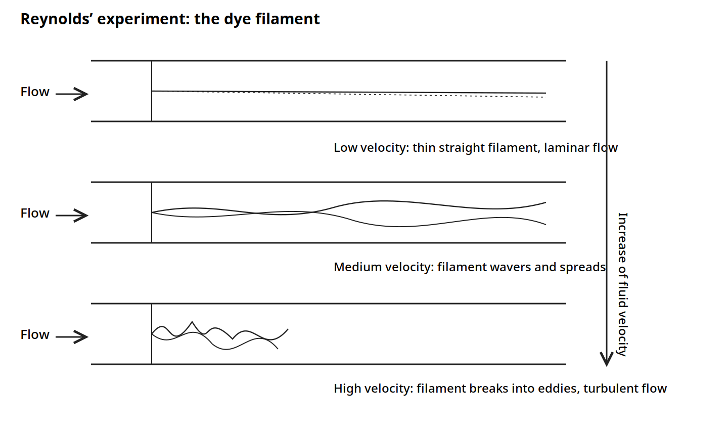
Figure 2.1: Reynolds' experiment. A dye filament stays thin and straight at low velocity, wavers and spreads as velocity rises, and breaks into eddies at high velocity. Reproduced from Ibarz, Fig. 3.1, p. 46.
Reynolds concluded that the instability could be predicted from the ratio of the kinetic forces and the viscous forces in the fluid stream. The kinetic forces tend to maintain the flow in its general direction, whereas the viscous forces tend to retard the motion and introduce eddies. The inertial force is proportional to the velocity pressure ρv², and the viscous drag is proportional to μv/D, where D is the diameter of the pipe. The ratio of these forces is ρvD/μ. That ratio is dimensionless, it is called the Reynolds number, and it is denoted by Re:
Re = Dvρ/μ
From a host of experimental measurements on fluid flow in pipes, Earle gives the boundaries as: for Re below 2100, streamline flow; for Re between 2100 and 4000, transition, where the pattern is unstable and any slight disturbance upsets it, although streamline flow can be maintained if there is no disturbance; and for Re above 4000, turbulent flow. Ibarz gives the same critical value of 2100 for Newtonian fluids, with a transition range above it, and the regime completely turbulent for values above 10,000. The difference between the two books is a matter of where fully developed turbulence is taken to begin, and this unit keeps both statements so the reader is not surprised to meet either number.
Worked example: is milk flow turbulent? (Earle Example 3.9)
Milk is flowing at 0.12 m³ per minute in a 2.5 cm diameter pipe. If the temperature of the milk is 21 °C, is the flow turbulent or streamline? The viscosity of milk at 21 °C is 2.1 cP, which is 2.1 x 10⁻³ Pa s, and the density is 1029 kg m⁻³. The diameter is 0.025 m and the cross sectional area is 4.9 x 10⁻⁴ m². The velocity is (0.12/60)/4.9 x 10⁻⁴ = 4.1 m s⁻¹. The Reynolds number is (0.025 x 4.1 x 1029)/(2.1 x 10⁻³) = 50,230. That is greater than 4000, so the flow is turbulent.
Diagram: Is milk flow turbulent? (Earle Example 3.9)
Milk at 21 °C, density 1029 kg m⁻³, viscosity 2.1 x 10⁻³ Pa s
↓
Flow 0.12 m³ per minute
Velocity 4.1 m s⁻¹
↓
Reynolds number 50,230, greater than 4000: turbulent
Diagram for Earle Example 3.9: milk at 4.1 m s⁻¹ in a 2.5 cm pipe is turbulent.
Because Re is dimensionless, its numerical value is the same whatever units are used, provided the units are consistent throughout. If centimetres were used instead of metres just in the diameter term, the value would be greater by a factor of 10, which would make nonsense of any deduction from the number.
Quick check
Water flows in a pipe at Re = 1500. Honey flows in the same pipe at Re = 50. Which flow is streamline, and which fluid has the higher viscosity relative to its speed?
Check your answer
Both are streamline, since both are below 2100. The honey has the lower Reynolds number, so viscous forces dominate more strongly in the honey flow.
2.8 Friction in pipes: the price of moving fluid
In Bernoulli's equation the symbol E_f denotes the energy loss due to friction in the pipe. That loss has been shown, both theoretically and experimentally, to be related to the Reynolds number for the flow. It is also proportional to the velocity pressure of the fluid and to a factor related to the smoothness of the surface over which the fluid is flowing.
If the wall friction is defined in terms of the velocity pressure, F/A = fρv²/2, where F is the friction force, A is the area over which it acts, and f is a coefficient called the friction factor, then an energy balance over a length L of straight horizontal pipe of diameter D gives the Fanning equation:
ΔP_f = (4fρv²/2)(L/D)
and the frictional loss of energy is E_f = ΔP_f/ρ = (4fv²/2)(L/D). The equation is also called the Fanning-Darcy equation, and it is used to calculate the pressure drop which occurs when liquids flow in pipes.
The factor f depends on the Reynolds number and on the roughness of the pipe. Earle's Fig. 3.8 plots experimental results showing that relationship. For low values of Re there is a simple relationship between f and Re, independent of the roughness of the pipe, because in streamline flow there is a stationary boundary layer at the wall and no liquid movement over any roughness at the wall. In streamline flow the friction factor can be predicted theoretically from the Hagen-Poiseuille equation:
f = 16/(Re), for 0 < (Re) < 2100
For smooth pipes in the range 3000 < (Re) < 100,000, the Blasius equation applies: f = 0.316/(Re)^0.25 in the Fanning form used by Earle. In the turbulent region a number of curves are shown, one for each roughness ratio, which is the ratio of the average height of the projections making up the roughness on the wall to the pipe diameter.
Some writers use values for f which differ from Earle's definition by numerical factors of 2 or 4, using the same symbol f, so when reading off values for f its definition in the particular context should always be checked. For example, a new factor f' = 4f removes the numerical factor from the Fanning equation. Ibarz uses the Darcy form, written as 4f, and that difference is the reason the two books' Moody diagrams look different while saying the same thing.
The roughness of a pipe is given in Earle's Table 3.1 as the roughness factor ε in metres:
Table 2.1: Relative roughness factors for pipes (Earle Table 3.1)
| Material | Roughness factor ε (m) | Material | Roughness factor ε (m) |
|---|---|---|---|
| Riveted steel | 0.001-0.01 | Galvanized iron | 0.0002 |
| Concrete | 0.0003-0.003 | Asphalted cast iron | 0.001 |
| Wood staves | 0.0002-0.003 | Commercial steel | 0.00005 |
| Cast iron | 0.0003 | Drawn tubing | Smooth |
Table 2.1: Roughness factors for pipes, Earle Table 3.1, p. 36.
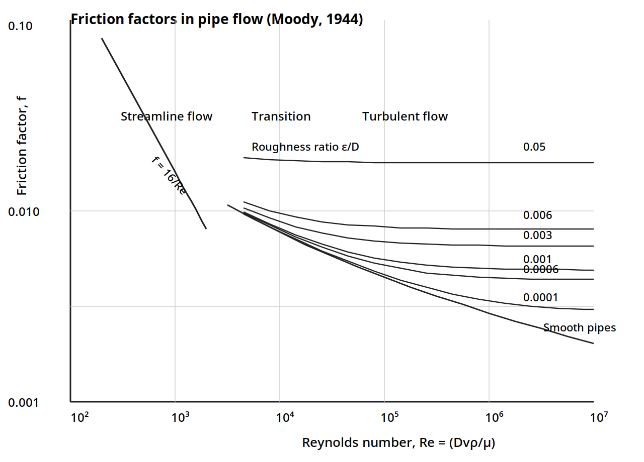
Figure 2.2: Friction factors in pipe flow. The laminar line is f = 16/Re; the turbulent curves are labelled by the roughness ratio ε/D. The curves are drawn from the Colebrook relation, which the book cites as the fit to these curves, with the laminar line exact; the individual curve positions are a faithful redrawing of the printed chart and are flagged as such in DIAGRAM-FLAGS.md. Reproduced from Earle, Fig. 3.8, p. 35, from Moody (1944) by permission.
Worked example: pressure drop for olive oil (Earle Example 3.10)
Calculate the pressure drop along 170 m of 5 cm diameter steel pipe through which olive oil at 20 °C is flowing at the rate of 0.1 m³ per minute. The viscosity of olive oil at 20 °C is 84 x 10⁻³ Pa s and the density is 910 kg m⁻³. The diameter is 0.05 m and the cross sectional area is 1.96 x 10⁻³ m². The velocity is (0.1/60)/1.96 x 10⁻³ = 0.85 m s⁻¹. The Reynolds number is (0.05 x 0.85 x 910)/(84 x 10⁻³) = 460, so the flow is streamline, and from Fig. 3.8 the friction factor is about 0.03, which agrees with the theoretical value 16/(Re) = 0.035 within chart reading accuracy. The pressure drop from the Fanning equation is ΔP = (4 x 0.03 x 910 x 0.85²/2) x (170/0.05) = 1.34 x 10⁵ Pa = 134 kPa.
2.9 The Moody diagram in Ibarz: the same chart, the other friction factor
Ibarz gives the same chart in the Darcy form, where the vertical axis is 4f, the Darcy friction factor. The chart covers Reynolds numbers from 10³ to 10⁸ and 4f from 0.008 to 0.1, with the zones marked as Laminar zone, Critical zone, Transition zone, Turbulent zone, and Rough pipings, complete turbulence. The laminar line is 4f = 64/Re. A dashed curve crosses the chart from the transition zone down to the smooth pipe curve. The two roughness curves labelled on the chart are ε/d = 0.000001 and ε/d = 0.000005.
The text beside the chart gives the working rules. For Reynolds numbers smaller than 2100, the variation of 4f with Re is linear, which agrees with the laminar equation. In the turbulent zone, the curves fit with a small error to the Colebrook equation. In the transition zone, for Reynolds numbers between 2100 and 4000, a relation that gives good results is f = 0.71 x 10⁻⁹(Re)². Another correlation frequently used for smooth pipes is 1/(4f)^0.5 = 1.80 log(Re/6.81). The practical way to calculate the friction factor is from the Moody diagram, where the friction factor is a function of the Reynolds number and the relative rugosity ε/d.
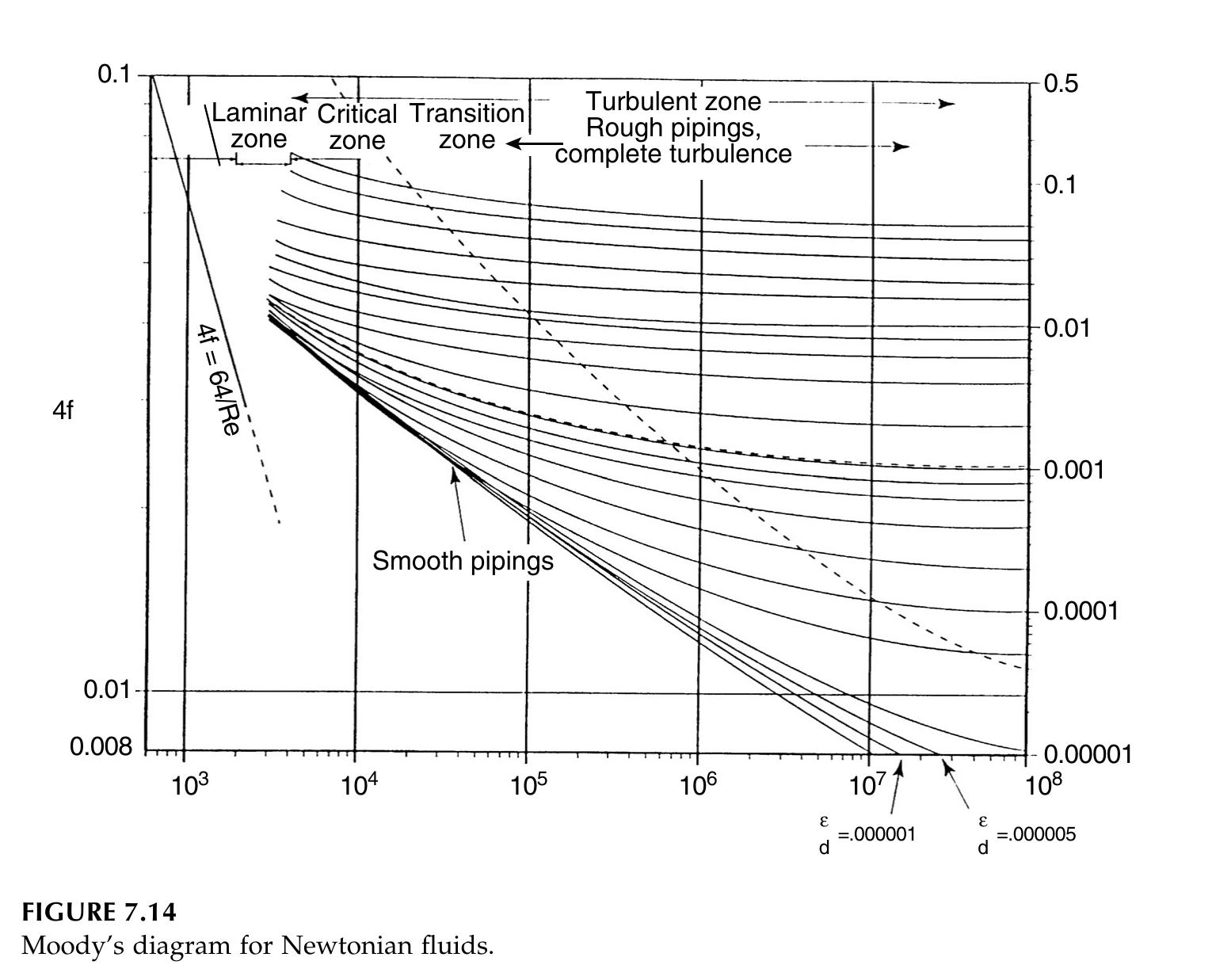
Figure 2.3: Moody's diagram for Newtonian fluids. The vertical axis is 4f, the Darcy friction factor, and the horizontal axis is the Reynolds number, both on log scales. The laminar line is 4f = 64/Re and is exact. The two roughness curves labelled on the book chart are ε/d = 0.000001 and ε/d = 0.000005. Reproduced from Ibarz, Fig. 7.14, p. 171.
Ibarz Table 7.1 gives the rugosity ε of pipe materials in millimetres. Note that Earle's Table 3.1 and Ibarz Table 7.1 give slightly different values for the same materials, because they come from different sources; use one table consistently within a calculation and say which one.
Table 2.2: Rugosity of pipes (Ibarz Table 7.1)
| Material | ε (mm) |
|---|---|
| Concrete | 0.3-3 |
| Cast iron | 0.26 |
| Asphalted cast iron | 0.12 |
| Galvanized iron | 0.15 |
| Wrought iron | 0.046 |
| Commercial steel | 0.046 |
| Riveted steel | 1-10 |
| Drain piping | 0.0015 |
Table 2.2: Rugosity of pipes, Ibarz Table 7.1, p. 187.
Quick check
A designer reads f = 0.005 from a chart that uses the Fanning definition, then uses it in an equation that expects the Darcy factor. What factor is wrong, and by how much?
Check your answer
The Darcy factor is 4f, so the Darcy value is 0.02, four times the Fanning value. Using 0.005 in a Darcy equation would understate the pressure drop by a factor of four.
2.10 Bends, valves and fittings: small pieces, large losses
When the direction of flow is altered or distorted, as when the fluid flows round bends in the pipe or through fittings of varying cross section, energy losses occur which are not recovered. The energy is dissipated in eddies and additional turbulence and finally lost in the form of heat. However, that energy must be supplied if the fluid is to be maintained in motion, in the same way as energy must be provided to overcome friction. Losses in fittings have been found to be proportional to the velocity head of the fluid, and the energy loss is expressed as:
E_f = kv²/2
where k has to be found for the particular fitting. Values of k for some fittings are given in Earle's Table 3.2, and a fuller set is given in Ibarz Table 7.3.
Energy is also lost at sudden changes in pipe cross section. At a sudden enlargement the loss is (v₁ - v₂)²/2, where v₁ is the velocity upstream and v₂ the velocity downstream. At a sudden contraction the loss is kv²/2, where k depends on the ratio of the pipe diameters, as in Earle's Table 3.3: for D₁/D₂ of 0.1, 0.3, 0.5, 0.7 and 0.9, k is 0.36, 0.31, 0.22, 0.11 and 0.02.
Table 2.3: Friction loss factors in fittings (Earle Table 3.2, selected values)
| Fitting | k |
|---|---|
| Valves, fully open: gate | 0.13 |
| Valves, fully open: globe | 6.0 |
| Valves, fully open: angle | 3.0 |
| Elbows: 90 degree standard | 0.74 |
| Elbows: medium sweep | 0.5 |
| Elbows: long radius | 0.25 |
| Tee, straight through | 0.5 |
| Entrance, large tank to pipe: sharp | 0.5 |
| Entrance, large tank to pipe: rounded | 0.05 |
Table 2.3: Friction loss factors in fittings, Earle Table 3.2, p. 37. Two further rows of the book table, the square elbow and the tee used as an elbow, could not be read reliably from the scanned page and are left out rather than guessed.
A globe valve, with k of 6.0, costs about forty six times as much energy as a fully open gate valve, with k of 0.13. That is why gate valves are used where the valve stays open, and globe valves where flow must be throttled. A sharp entrance costs ten times a rounded one.
Ibarz gives the same losses as equivalent lengths of straight pipe. A fictitious length of straight pipe is added to the actual length, such that the friction due to the fictitious pipe is the same as that from the fitting. Since the fitting loss kv²/2 equals the pipe friction loss, k can be replaced by 4fL_e/D, where L_e is the equivalent length. Table 7.2 gives the equivalent length in pipe diameters for turbulent flow only.
Table 2.4: Equivalent length of different fittings, for turbulent flow only (Ibarz Table 7.2)
| Fitting | L_e/d |
|---|---|
| 45 degree elbow standard | 15 |
| 90 degree elbow standard | 30 |
| 90 degree elbow long radius | 20 |
| 180 degree return elbow | 75 |
| Tee standard, used as elbow, central entrance | 90 |
| Tee standard, used as elbow, entrance by lateral branch | 60 |
| Tee standard, straight passing | 20 |
| Check valve, fully open | 300 |
| Angle valve, fully open | 170 |
| Gate valve, fully open | 7 |
| Gate valve, 1/4 open | 900 |
| Gate valve, 1/2 open | 200 |
| Gate valve, 3/4 open | 40 |
| Ordinary entrance | 16 |
| Borda entrance | 30 |
| Rounded entrance, joints, couplings | Negligible |
Table 2.4: Equivalent length of different fittings, Ibarz Table 7.2, p. 176. Source given in the book: Levenspiel, Flujo de Fluidos, Intercambio de Calor, Reverte, Barcelona, 1993.
A gate valve that is only a quarter open is equivalent to 900 pipe diameters of straight pipe, while the same valve fully open is only 7. A half closed gate valve is a very expensive way to throttle a flow.
Table 2.5: Resistance factors k (Ibarz Table 7.3, selected values)
| Fitting | k | Fitting | k |
|---|---|---|---|
| 45 degree elbow standard | 0.35 | Gate valve, fully open | 0.17 |
| 45 degree elbow great curvature | 0.20 | Gate valve, 3/4 open | 0.90 |
| 90 degree elbow standard | 0.75 | Gate valve, 1/2 open | 4.50 |
| 90 degree elbow great curvature | 0.45 | Gate valve, 1/4 open | 24.00 |
| 90 degree elbow small curvature | 1.30 | Check valve, fully open | 9.00 |
| 180 degree curve | 1.50 | Check valve, 1/2 open | 36.0 |
| Tee standard, with closed fork | 0.40 | Check valve, 1/4 open | 112.0 |
| Tee standard, used as elbow | 1.00 | Diaphragm valve, fully open | 2.30 |
| Tee standard, with flow division | 1.00 | Angle valve, fully open | 2.00 |
| Threaded joints | 0.04 | Bottom valve | 15.0 |
| Entrance, trumpet shaped | 0.78 | Entrance, sharp edges | 0.50 |
| Entrance, slightly rounded | 0.23 | Entrance, fully rounded | 0.04 |
| Exit, trumpet shaped, sharp edges or rounded | 1.00 | Retention valve, ball | 70.00 |
Table 2.5: Resistance factors k, Ibarz Table 7.3, p. 178. Selected values; the full table in the book also gives ball and butterfly valve factors at 5, 10, 20, 40 and 60 degrees closed, and flowmeter factors for disk, piston, revolving and turbine meters.
These resistance factors are valid only for fluids with Newtonian behaviour. For non-Newtonian fluids the available information is limited. Steffe and co-workers reported that the factors increase as the generalized Reynolds number decreases, with expressions for three way valves, tee fittings and 90 degree elbows that depend on the generalized Reynolds number raised to a negative power.
Pressure drops through equipment such as banks of tubes in heat exchangers, or beds of packed solids, are not easy to calculate even if the properties of the solids are well known, and accurate pressure drop information generally needs experimental measurement. Two useful generalizations hold: pressure drops through equipment are in general proportional to the square of the velocity, and power requirements are proportional to the product of the pressure drop and the mass rate of flow, that is to the cube of the velocity. Doubling the flow rate through a pipe roughly doubles the pressure drop four times and the power eight times.
Practical note: when a pump cannot keep up, the first thing to check is not the pump but the line: a half closed gate valve, a globe valve left in a line that should have a gate valve, or a sharp entrance can cost more head than a hundred metres of straight pipe.
2.11 Measuring pressure and flow
Two practical aspects of fluid flow are measurement and the production of flow by pumps and fans. Only by measuring variables such as pressure and velocity can the flow of the fluid be controlled.
The simplest method of measuring pressure is the piezometer tube, a tube containing the fluid under pressure in which the fluid is allowed to rise to a height that corresponds to the excess of the pressure over its surroundings. The head can be related to the pressure by P = ρZg. A development of the piezometer is the U-tube, in which another fluid is introduced which must be immiscible with the fluid whose pressure is being measured. The unknown pressure is then equal to the difference between the levels of the measuring fluid in the two arms of the U-tube.
Worked example: vacuum in an evaporator (Earle Example 4.1)
The pressure in a vacuum evaporator was measured and found to be less than atmospheric pressure by 25 cm of mercury, as measured in a U-tube. Calculate the vacuum and the absolute pressure in the evaporator. The atmospheric pressure is 75.4 cm of mercury and the specific gravity of mercury is 13.6. The vacuum is P = 13.6 x 1000 x 0.25 x 9.81 = 33.4 kPa. The atmospheric pressure is 13.6 x 1000 x 0.754 x 9.81 = 100.6 kPa, so the absolute pressure in the evaporator is 100.6 - 33.4 = 67.2 kPa.
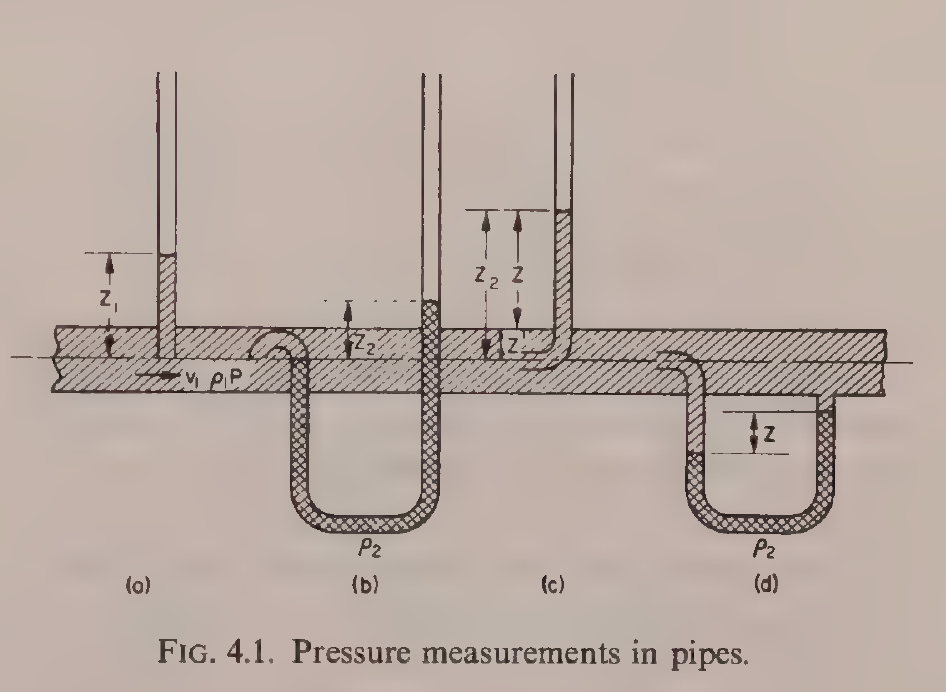
Earle Fig. 4.1: Pressure measurements in pipes: (a) piezometer, (b) U-tube, (c) Pitot tube, (d) Pitot-static tube. Reproduced from Earle, Fig. 4.1, printed p. 39.
The most common pressure measuring instrument is the Bourdon tube pressure gauge. A coiled tube tends to straighten itself when subjected to internal pressure, and the degree of straightening is directly related to the difference between the pressure inside the tube and the pressure outside it. A bellows gauge works on a similar principle, with unknown pressure acting against a spring.
Velocity is measured with a Pitot tube, a tube bent so that its mouth faces directly into the flow. The pressure in the tube gives a measure of the velocity head. Combined with a piezometer tube across a common manometer, the differential head measures directly the velocity head of the flowing liquid. That arrangement is known as a Pitot-static tube and is extensively used in measuring flow velocities.
Worked example: air velocity in a duct (Earle Example 4.2)
Air at 0 °C is flowing through a duct in a chilling system. A Pitot-static tube is inserted and the differential pressure head measured is 0.8 mm of water. Calculate the velocity of the air. The density of air at 0 °C is 1.3 kg m⁻³. Converting the head into an equivalent head of air, 0.8 mm of water is 0.8 x 10⁻³ x (1000/1.3) = 0.62 m of air. From the velocity head relation, v²/2 = 0.62 x 9.81, so v = 3.5 m s⁻¹.
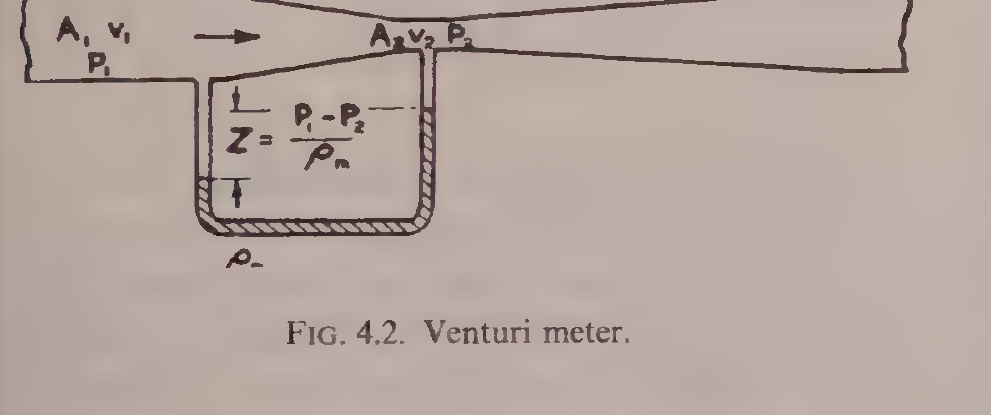
Earle Fig. 4.2: Venturi meter. Reproduced from Earle, Fig. 4.2, printed p. 41.
Another method uses the pressure drop across a constriction. In a venturi meter, a gradual constriction reduces the area of flow from A₁ to A₂, the velocity rises and the static pressure falls in accordance with Bernoulli's equation. Joining the two sections to a U-tube manometer measures the differential head directly. In practice energy losses occur between the two measuring points, and a coefficient C is introduced to allow for this. In a properly designed venturi meter C lies between 0.95 and 1.0. An orifice meter works on the same principle, but instead of a tapered tube a plate with a hole in the centre is inserted in the pipe. The same equations hold, but the orifice discharge coefficient is smaller, and orifices have much greater pressure losses than venturi meters, although they are easier to construct and to insert in pipes. Other meters in use are propeller meters, impact meters and rotameters, in which a rotor disc is supported against gravity in a tapered vertical tube and rises to a height that depends on the flow velocity.
Quick check
A venturi meter and an orifice meter both measure flow from a pressure drop. Which one wastes more energy, and why would anyone choose it?
Check your answer
The orifice meter wastes more energy, because the sharp plate causes a larger permanent pressure loss. It is chosen because it is cheap and easy to fit into an existing pipe.
2.12 Pumps and fans: putting energy into the fluid
In pumps and fans, mechanical energy from some other source is converted into pressure or velocity energy in a fluid. The food technologist is not concerned with the details of pump design, but should know what classes of pump are used and something about their characteristics. The efficiency of a pump is the ratio of the energy supplied by the motor to the increase in velocity and pressure energy given to the fluid.
Positive displacement pumps draw the fluid in and then force it through the outlet. The types are reciprocating piston pumps; gear pumps, in which the fluid is enmeshed in rotating gears and forced through the pump; and rotary pumps, in which rotating vanes draw in and discharge fluid through a system of valves. Positive displacement pumps can develop high pressure heads, but they cannot tolerate throttling or blockages in the discharge.
Jet pumps produce a high velocity jet in a venturi nozzle, converting the energy of the fluid into velocity energy. That produces a low pressure area, causing the surrounding fluid to be drawn into the throat, and the combined fluids are then discharged. Jet pumps are used for difficult materials which cannot be handled satisfactorily in a mechanical pump, and as vacuum pumps. They have relatively low efficiencies but no moving parts and a low initial cost, and they can develop only low heads per stage.
Air-lift pumps introduce air or gas into a liquid to impart energy to it. Examples are air introduced to pump water from an artesian well, air introduced above a liquid in a pressure vessel to discharge it, vapours produced in the column of a climbing film evaporator, and air blown up through a bed of powder to convey it in fluidized form. Air-lift pumps and air blowing are inefficient, but they are convenient for materials which will not pass easily through the ports, valves and passages of other types of pumps.
Propeller pumps and fans impart energy with a propeller. They are used extensively to mix the contents of tanks and in pipelines to mix and convey the fluid. Propeller fans are common and have high efficiencies, but they can only be used for low heads, in the case of fans only a few centimetres of water.
Centrifugal pumps and fans convert rotational energy into velocity and pressure energy. The fluid is taken in at the centre of a bladed rotor and passes out along the spinning rotor, acquiring energy of rotation, which is then converted into velocity and pressure energy at the periphery of the disc. Centrifugal pumps can develop moderate heads of up to 20 m of water, and they can deliver very large quantities of fluids with high efficiency.
Gould adds the plant view. Pumps and pumping are one of the most important aspects of nearly all food processing operations, and some consider pumps the heart of many food operations. Pumps are classified into positive displacement pumps and centrifugal pumps, and each class is used in most food plants. All food contact surfaces of food pumps should be of 304 stainless steel or equivalent. One key feature to look for beyond maintenance is the Cleaned In Place feature: tearing down pumps to clean them is costly in manpower and costly in lost production time.
Ibarz sets out the pump quantities that matter for design. The total head a pump can develop is the difference between the discharge head and the suction head. The net positive suction head, NPSH, decides whether the pump cavitates. Cavitation is a phenomenon produced when the pressure at some point of the pump falls to the vapour pressure of the liquid, so that vapour bubbles form and then collapse. It causes a decrease of the suction and discharge pressures of the pump, which can empty it, and it damages the pump. To avoid cavitation, the available NPSH, which depends on the placement of the pump and the properties of the liquid, must be greater than the required NPSH, which is characteristic of each pump and is given by the manufacturer as a function of the pump design and its rotation speed. Cavitation appears when the pressure at the suction point falls below the vapour pressure. It can be avoided by increasing the pressure at the suction point, by lowering the height at which the pump is placed, or by decreasing the vapour pressure of the liquid, for example by cooling it. The pump power is the mass flow rate times the mechanical energy per unit mass supplied by the pump, and the real power is the theoretical power divided by the pump efficiency.
For a given centrifugal pump, the capacity varies with its rotational speed, the pressure developed varies as the square of the rotational speed, and the power required varies as the cube of the rotational speed. The same proportional relationships apply to centrifugal fans, and they are often called the fan laws.
Earle's Fig. 4.4 shows the characteristic curves for a centrifugal pump, reproduced with permission from Coulson and Richardson, Chemical Engineering, 2nd edition, fig. 6.15. The horizontal axis is capacity in m³ s⁻¹ from 0 to 0.030, and the vertical axis is total head in metres from 0 to 45. The chart carries three families of curves: impeller diameter curves from 90 mm to 150 mm, efficiency contours from 50% to 77%, and power curves from 1 kW to 8 kW, with an economical range marked at 57.5 Hz. The chart below is the book's own figure, with the same axes, the same impeller diameters, the same efficiency values and the same power values.
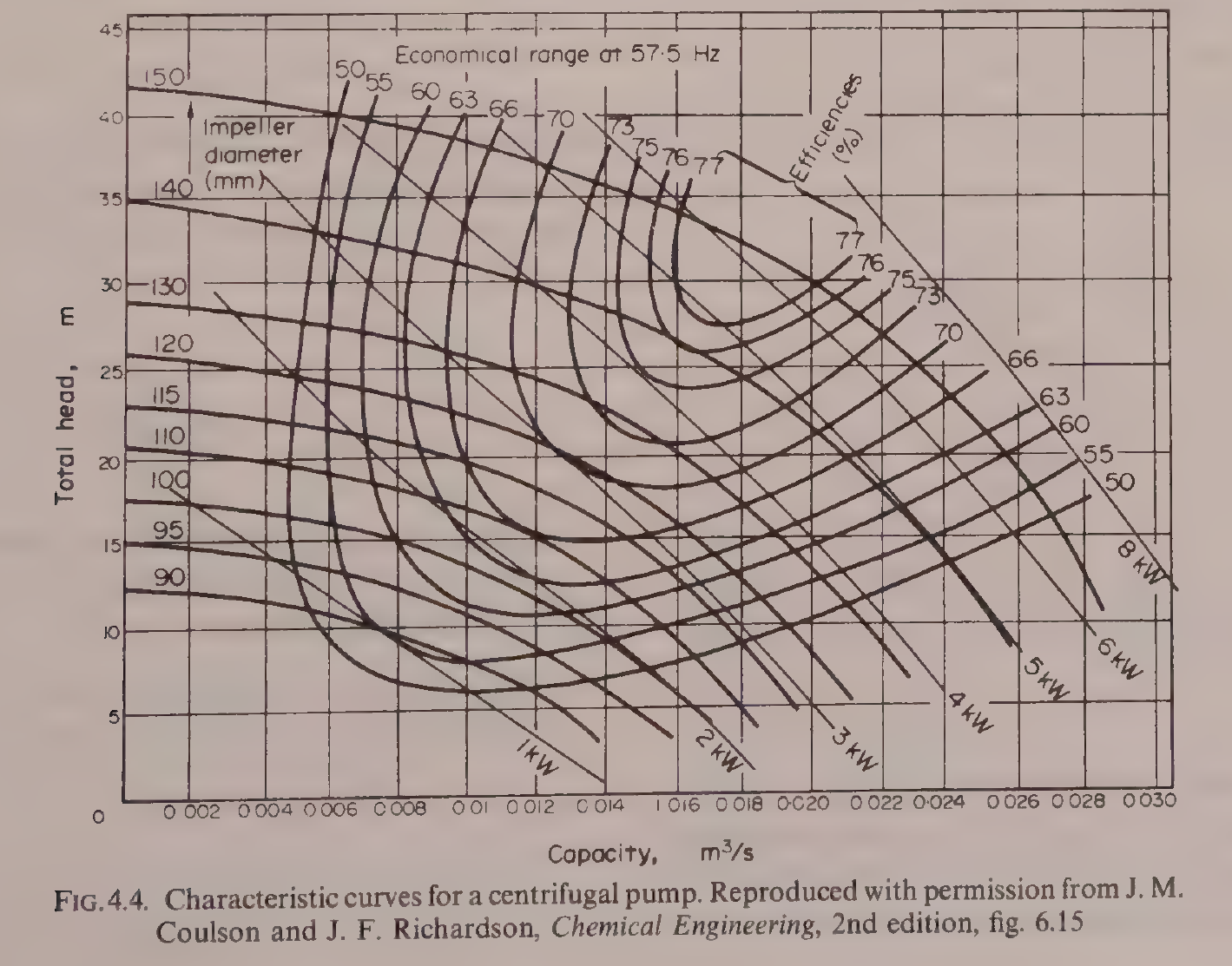
Figure 2.4: Characteristic curves for a centrifugal pump. Axes, impeller diameters (90 to 150 mm), efficiency contours (50 to 77%) and power curves (1 to 8 kW) are as in the book. Reproduced from Earle, Fig. 4.4, p. 43, reproduced with permission from J. M. Coulson and J. F. Richardson, Chemical Engineering, 2nd edition, fig. 6.15.
To use the chart, find the duty point where the required capacity and the required head meet, then read off the impeller diameter that passes through that point, the efficiency contour that encloses it, and the power curve that passes through it. A pump running far from its economical range wastes power and wears faster. That is the practical meaning of the chart: match the pump to the duty, do not just buy a big one.
Brennan's Appendix I gives the same fluid flow formulae in compact form, including flow through equipment and fluidization, and it is the reference to reach for when a quick formula is needed without working through a chapter.
Try it yourself: Take a garden hose and a bucket. Time how long it takes to fill the bucket with the tap half open, then fully open. Measure the hose diameter. Work out the velocity and the Reynolds number for water at about 20 °C, with a viscosity of 1 x 10⁻³ Pa s and a density of 1000 kg m⁻³. Then kink the hose part way: the flow drops far more than the kink looks worth. That is a fitting loss, and you have just measured it with a bucket and a watch.
Key ideas to carry forward
- A fluid in food engineering covers liquids, gases and fluidized solids, because they obey many of the same laws.
- Pressure in a still liquid is P = Zρg: it depends only on depth and density, not on the shape of the vessel.
- The continuity equation A₁v₁ = A₂v₂ says volume flow is the same at every section of a pipe, so velocity rises where the pipe narrows.
- Bernoulli's equation Zg + v²/2 + P/ρ = k is the energy balance for flow, and it can be written as energies, as pressures, or as heads.
- Viscosity is the resistance to relative movement of adjacent layers, given by F/A = μv/Z. Water is about 1 x 10⁻³ N s m⁻², olive oil about 100 x 10⁻³, and molasses about 7.
- Newtonian fluids obey τ = μ(dv/dZ). Non-Newtonian fluids follow the power law: pseudoplastic fluids such as tomato purée thin with shear, dilatant fluids such as gritty slurries thicken with shear, and some fluids need a yield stress before they flow at all.
- The Reynolds number Re = Dvρ/μ decides the flow regime: below 2100 streamline, between 2100 and 4000 transition, above 4000 turbulent in Earle, with Ibarz taking fully turbulent flow above 10,000.
- Friction loss in a straight pipe follows the Fanning equation ΔP_f = (4fρv²/2)(L/D). In streamline flow f = 16/(Re). In turbulent flow f comes from the Moody diagram, as a function of Re and the roughness ratio ε/D.
- Earle's friction factor f and Ibarz's 4f differ by a factor of four: the Darcy factor is 4f. Always check which definition a chart or a table uses.
- Fitting losses are kv²/2, or the equivalent length of straight pipe. A globe valve costs far more than a gate valve, and a half closed gate valve costs far more than either.
- Pressure is measured with piezometer tubes, U-tubes and Bourdon gauges. Flow is measured with Pitot-static tubes, venturi meters, orifice meters and rotameters.
- Pumps divide into positive displacement, jet, air-lift, propeller and centrifugal types. A centrifugal pump is chosen from its characteristic curves, matching capacity, head, efficiency and power to the duty.
- Cavitation happens when the pressure at the pump suction falls to the vapour pressure of the liquid. The available NPSH must be greater than the required NPSH.
Glossary
Fluid
A substance that flows, including liquids, gases and fluidized solids. Food tech example: milk, fruit juice, syrup, air and flour all count as fluids in a food factory.
Fluid statics
The study of fluids at rest, including the pressure a still liquid exerts. Food tech example: the pressure at the bottom of a storage tank, which depends only on the depth of liquid.
Fluid dynamics
The study of fluids in motion. Food tech example: milk flowing through a pasteurizer pipe.
Pressure head
A pressure expressed as the height of a column of a given fluid that would produce it. Food tech example: atmospheric pressure is about 10.2 m of water.
Gauge pressure
Pressure measured above atmospheric pressure as the datum. Food tech example: a retort gauge reading 100 kPa means 100 kPa above the air outside.
Continuity equation
The mass balance for flow in a pipe: for an incompressible fluid, A₁v₁ = A₂v₂, so the volume flow is the same at every section. Food tech example: milk speeding up as it passes from a wide pipe into a narrow one.
Bernoulli's equation
The energy balance for frictionless flow: Zg + v²/2 + P/ρ is constant along the flow. Food tech example: the pressure falling in a pipe where it narrows and the velocity rises.
Velocity head
The kinetic energy term of Bernoulli's equation written as a height, v²/2g. Food tech example: the head a Pitot tube measures to find the velocity of air in a duct.
Viscosity
The property of a fluid that resists the relative movement of adjacent layers, measured in N s m⁻². Food tech example: honey at about 7 N s m⁻² pouring far more slowly than water at about 1 x 10⁻³ N s m⁻².
Newtonian fluid
A fluid that obeys Newton's law of viscosity, with a constant viscosity whatever the shear rate. Food tech example: water, milk and fruit juice.
Non-Newtonian fluid
A fluid whose apparent viscosity changes with the shear rate. Food tech example: tomato purée, which flows more easily the harder it is stirred.
Pseudoplastic
A non-Newtonian fluid whose apparent viscosity falls as the shear rate rises. Food tech example: tomato purée.
Dilatant
A non-Newtonian fluid whose apparent viscosity rises as the shear rate rises. Food tech example: a gritty slurry of crystallized sugar solution.
Yield stress
The minimum shear stress that must be applied before a fluid starts to flow. Food tech example: a thick paste that stays put in a pipe until the pump pressure passes a threshold.
Reynolds number
The dimensionless ratio of inertial to viscous forces in a flowing fluid, Re = Dvρ/μ. Food tech example: milk in a pipe at Re = 50,230, which is turbulent flow.
Streamline flow
Smooth flow in parallel layers with no mixing across the flow, also called laminar flow. Food tech example: olive oil flowing slowly in a pipe at Re = 460.
Turbulent flow
Flow with eddies and mixing across the direction of flow. Food tech example: milk flowing fast in a pipe at Re = 50,230.
Friction factor
The coefficient f that relates the wall friction in a pipe to the velocity pressure of the fluid. Food tech example: f = 16/(Re) in streamline flow, read from the Moody diagram in turbulent flow.
Moody diagram
A log-log chart giving the friction factor as a function of Reynolds number and pipe roughness. Food tech example: finding f for olive oil in a steel pipe from Re and the roughness ratio.
Roughness ratio
The ratio of the average height of the roughness on a pipe wall to the pipe diameter, ε/D. Food tech example: commercial steel at ε = 0.00005 m, which is smooth beside riveted steel at up to 0.01 m.
Equivalent length
A length of straight pipe that would give the same friction loss as a fitting. Food tech example: a fully open gate valve equal to 7 pipe diameters, and the same valve a quarter open equal to 900.
Pitot tube
A tube facing into a flow that measures the velocity head. Food tech example: measuring the velocity of air in a chilling duct as 3.5 m s⁻¹.
Venturi meter
A flow meter that measures the pressure drop across a gradual constriction in a pipe. Food tech example: measuring milk flow without a moving part in the pipe.
Positive displacement pump
A pump that draws fluid in and forces it out through the outlet, such as a piston, gear or rotary pump. Food tech example: a gear pump moving thick jam that a centrifugal pump could not handle.
Centrifugal pump
A pump that converts rotational energy into velocity and pressure energy with a spinning bladed rotor. Food tech example: the standard pump for moving milk and water around a factory.
Cavitation
The formation and collapse of vapour bubbles when the pressure in a pump falls to the vapour pressure of the liquid. Food tech example: a pump that loses suction and rattles because it is placed too high above the supply tank.
NPSH
Net positive suction head, the head available at a pump suction above the vapour pressure of the liquid. Food tech example: the available NPSH must be greater than the required NPSH given by the pump maker, or the pump will cavitate.
References
- Earle, R. L., Unit Operations in Food Processing, 2nd edition, Pergamon Press, 1983. Chapter 3, Fluid-Flow Theory, including Examples 3.1 to 3.10, Figures 3.1 to 3.8 and Tables 3.1 to 3.3, and Chapter 4, Fluid-Flow Applications, including Examples 4.1 to 4.3 and Figures 4.1 to 4.4.
- Ibarz, Albert, and Barbosa-Canovas, Gustavo V., Unit Operations in Food Engineering, CRC Press, 2003. Chapter 3, Introduction to Transport Phenomena, including Figures 3.1 and 3.2; Chapter 4, Molecular Transport of Momentum, Energy, and Mass, including Newton's law of viscosity, Fourier's law and Fick's law; and Chapter 7, Transport of Fluids through Pipes, including Figures 7.13 and 7.14 and Tables 7.1, 7.2 and 7.3.
- Brennan, J. G., Butters, J. R., Cowell, N. D., and Lilly, A. E. V., Food Engineering Operations, Elsevier, 1969. Appendix I, Fluid Flow Formulae.
- Gould, Wilbur A., Unit Operations for the Food Industries, CTI Publications, 1996. Chapter 11, Pumps and Pumping.
- Moody, L. F. (1944), as reproduced in Earle, Fig. 3.8, and in Ibarz, Fig. 7.14.
- Coulson, J. M., and Richardson, J. F., Chemical Engineering, 2nd edition, as reproduced in Earle, Fig. 4.4.
Unit 3: Heat Transfer and Heat Exchangers
Note
Unit 3: Heat Transfer and Heat Exchangers
Heat a cold store wall from the outside and the cold leaks away, slowly, through brick, concrete and cork. Heat a pan of soup and the steam in the jacket gives up its heat through steel, into the soup, and the soup warms. Cool milk in a plate exchanger and the cold brine takes the heat away through thin steel plates, square metre after square metre. The same few rules govern all three, and this unit is about those rules, the numbers that go with them, and the machines built around them.
Questions to think about
- What drives heat to flow, and what holds it back?
- Why does a steel bolt through an insulated wall carry most of the heat?
- What is the difference between thermal conductivity and thermal conductance?
- Why is the coldest part of a can the hardest part to heat, and how do engineers allow for it?
- What is an overall heat transfer coefficient, and which resistance controls it?
- Why is countercurrent flow better than parallel flow in a heat exchanger?
- How do you size a heat exchanger from four temperatures and two flow rates?
3.1 Heat transfer is everywhere in food processing
Heat transfer is an operation that occurs repeatedly in the food industry. Whether it is called cooking, baking, drying, sterilizing or freezing, heat transfer is part of the processing of almost every food. An understanding of the principles which govern heat transfer is essential to an understanding of food processing.
Heat transfer is a dynamic process in which heat is transferred spontaneously from one body to another cooler body. The rate of heat transfer depends on the differences in temperature between the bodies: the greater the difference in temperature, the greater the rate of heat transfer. Temperature difference between the source of heat and the receiver of heat is therefore the driving force in heat transfer. The heat passing from one body to another travels through some medium which in general offers resistance to the heat flow. Both factors, the temperature difference and the resistance to heat flow, affect the rate of heat transfer, and they are connected by the general equation:
rate of transfer = driving force / resistance
For heat transfer, the rate of heat transfer equals the temperature difference divided by the heat flow resistance of the medium. During processing, temperatures may change and therefore the rate of heat transfer will change. That is called unsteady-state heat transfer, in contrast to steady-state heat transfer, when the temperatures do not change. An example of unsteady-state heat transfer is the heating and cooling of cans in a retort to sterilize the contents.
Heat can be transferred in three ways. In conduction, molecular energy is directly exchanged from the hotter to the cooler regions, the molecules with greater energy communicating some of their energy to neighbouring molecules with less energy. An example is the heat transfer through the solid walls of a refrigerated store. Radiation is the transfer of heat energy by electromagnetic waves, which transfer heat from one body to another in the same way as light waves transfer light energy. An example is a foodstuff passed below a bank of red hot electric resistance heaters. Convection is the transfer of heat by the movement of groups of molecules in a fluid, moved by density changes or by forced motion of the fluid. An example is cooking in a jacketed pan: without a stirrer, density changes cause heat transfer by natural convection, and with a stirrer the convection is forced. In general, heat is transferred in solids by conduction and in fluids by conduction and convection, while radiation occurs through open space. In practice the three types may occur together. For calculations it is often best to consider the mechanisms separately, and then to combine them where necessary.
Quick check
A loaf bakes in an oven with hot air blowing round it and red hot elements above it. Name the three mechanisms at work.
Check your answer
Conduction through the crust and crumb, convection from the moving hot air to the loaf surface, and radiation from the red hot elements to the loaf.
3.2 Conduction: Fourier's law and the slab
In heat conduction, the general rate equation can be applied directly. The driving force is the temperature difference per unit length of heat transfer path, also known as the temperature gradient. Instead of resistance to heat flow, its reciprocal, called the conductance, is used. The equation becomes:
rate of heat transfer = driving force x conductance
dQ/dθ = kA(dt/dx)
where dQ/dθ is the rate of heat transfer, the quantity of heat energy transferred per unit time, A is the area of cross section of the heat flow path, dt/dx is the temperature gradient, and k is the thermal conductivity of the medium. That equation is known as the Fourier equation for heat conduction. Heat flows from a hotter to a colder body, in the direction of the negative temperature gradient, so a minus sign should appear in the Fourier equation. In simple problems the direction of heat flow is obvious and the minus sign is considered confusing rather than helpful, so it has not been used.
Thermal conductivity is a property of the material. It does change slightly with temperature, but in many applications it can be regarded as a constant for a given material. In general, metals have a high conductivity, in the region of 50 to 400 J m⁻¹ s⁻¹ °C⁻¹. Most foodstuffs contain a high proportion of water, and as the thermal conductivity of water is about 0.7 J m⁻¹ s⁻¹ °C⁻¹ above 0 °C, thermal conductivities of foods are in this range. Ice has a substantially higher thermal conductivity than water, about 2.3 J m⁻¹ s⁻¹ °C⁻¹, so the thermal conductivity of frozen foods is higher than that of foods at normal temperatures. Most dense non-metallic materials have thermal conductivities of 0.5 to 2 J m⁻¹ s⁻¹ °C⁻¹. Insulating materials such as foamed plastics, cork and expanded rubber are in the range 0.038 to 0.052 J m⁻¹ s⁻¹ °C⁻¹, close to the conductivity of air, which is 0.024 J m⁻¹ s⁻¹ °C⁻¹ at 0 °C. Some newer insulating materials have thermal conductivities as low as 0.026 J m⁻¹ s⁻¹ °C⁻¹.
If a slab of material has two faces at different temperatures t₁ and t₂, heat flows from the face at the higher temperature to the other face. Under steady temperature conditions the rate of heat transfer is constant, and the Fourier equation becomes:
q = kA(t₁ - t₂)/x = kAΔt/x = (k/x)AΔt
where x is the thickness of the slab. That is the basic equation for simple heat conduction, and it can be used to calculate the rate of heat transfer through a uniform wall if the temperature difference across it and the thermal conductivity of the wall material are known.
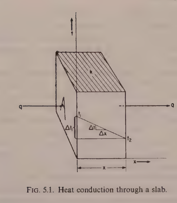
Figure 3.1: Heat conduction through a slab. Heat q flows from the face at temperature t₁ to the face at temperature t₂, across a thickness x, through a material of thermal conductivity k. Reproduced from Earle, Fig. 5.1, p. 48.
Worked example: heat through a cork slab (Earle Example 5.1)
A cork slab 10 cm thick has one face at -12 °C and the other face at 21 °C. If the mean thermal conductivity of cork in this temperature range is 0.042 J m⁻¹ s⁻¹ °C⁻¹, what is the rate of heat transfer through 1 m² of wall? The temperature difference is 21 - (-12) = 33 °C, the area is 1 m², k is 0.042 and x is 0.1 m. The rate is q = (0.042/0.1) x 1 x 33 = 13.9 J s⁻¹.
Quick check
Two walls have the same thickness and the same temperature difference. One is brick with k = 0.69, the other is cork with k = 0.043. Which passes more heat, and by what factor?
Check your answer
The brick wall, by a factor of 0.69/0.043, which is about 16 times as much heat.
3.3 Conductances in series and in parallel
The heat conductance is the quantity of heat that will pass in unit time, through unit area of a specified thickness of material, under unit temperature difference. It is C = k/x, with units J m⁻² s⁻¹ °C⁻¹. Conductance relates to the actual thickness of a given material, while conductivity relates only to unit thickness. That distinction matters whenever a wall is made of more than one layer.
Frequently, in heat conduction, heat passes through several consecutive layers of different materials. For example, in a cold store wall, heat might pass through brick, plaster, wood and cork. In the steady state, the same quantity of heat per unit time must pass through each layer. If the areas are the same, the temperature drops across the layers add, and the result is:
q = UAΔt, where 1/U = x₁/k₁ + x₂/k₂ + x₃/k₃ + ...
Here U is called the overall conductance for the combined layers. The same form as the single slab equation, extended to a composite slab.
Worked example: a cold store wall (Earle Example 5.2)
A cold store has a wall comprising 11 cm of brick on the outside, then 7.5 cm of concrete and then 10 cm of cork. The mean temperature within the store is maintained at -18 °C and the mean temperature of the outside surface of the wall is 18 °C. Calculate the rate of heat transfer through the wall and the temperature at the interface between cork and concrete. The thermal conductivities are for brick, concrete and cork, respectively, 0.69, 0.76 and 0.043 J m⁻¹ s⁻¹ °C⁻¹.
For brick, x₁/k₁ = 0.11/0.69 = 0.16. For concrete, x₂/k₂ = 0.075/0.76 = 0.10. For cork, x₃/k₃ = 0.10/0.043 = 2.33. The sum is 1/U = 0.16 + 0.10 + 2.33 = 2.6, so U = 0.38 J m⁻² s⁻¹ °C⁻¹. The temperature difference is 18 - (-18) = 36 °C, so the heat flow is q = UAΔt = 0.38 x 1 x 36 = 13.7 J s⁻¹ per m² of wall. For the cork layer, q = AΔt₃k₃/x₃, so 13.7 = 1 x Δt₃ x (1/2.33), giving Δt₃ = 32 °C. That is the difference between the cork and concrete interface and the inside surface of the cork, so the interface temperature is -18 + 32 = 14 °C.
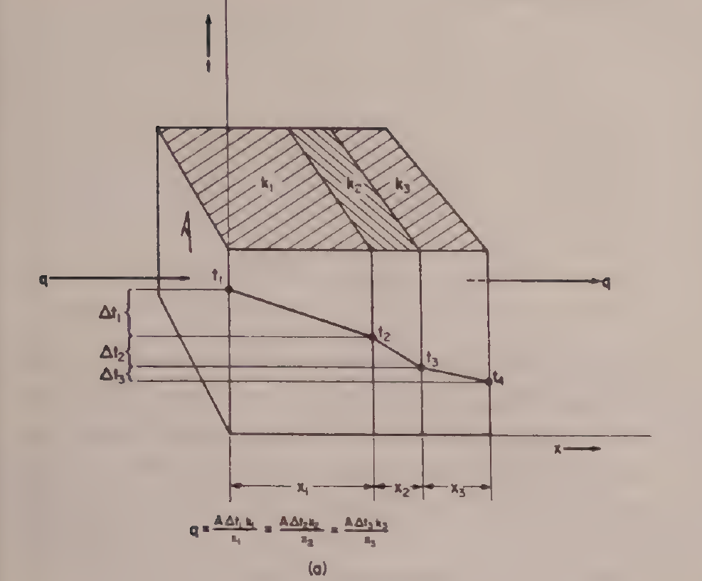
Earle Fig. 5.2(a): Heat conductances in series. Reproduced from Earle, Fig. 5.2(a), printed p. 49.
Notice where the resistance sits: the cork contributes 2.33 of the total 2.6, which is about 90% of the resistance. The brick and the concrete hardly matter. That is the point of the example, and it is a pattern that returns in every heat transfer calculation: find the largest resistance, because it controls the result.
Heat conductances in parallel are the opposite case. The material surfaces are parallel to the direction of heat transfer, so the heat passes through each material at the same time instead of through one and then the next. An example is the insulated wall of a refrigerator or an oven, in which the walls are held together by bolts. The bolts are in parallel with the direction of heat transfer through the wall: they carry most of the heat transferred and thus account for most of the losses.
Worked example: steel bolts in an oven wall (Earle Example 5.3)
The wall of a bakery oven is built of insulating brick 10 cm thick with a thermal conductivity of 0.22 J m⁻¹ s⁻¹ °C⁻¹. Steel reinforcing members penetrate the brick, and their total area of cross section represents 1% of the inside wall area. The thermal conductivity of the steel is 45 J m⁻¹ s⁻¹ °C⁻¹. Calculate the relative proportions of the total heat transferred through the wall by the brick and by the steel, and the heat loss for each m² of oven wall if the inner side is at 230 °C and the outer side is at 25 °C.
The temperature difference is the same for brick and steel, and the thickness is the same. For the brick, through 0.99 m²: q = 0.99 x (230 - 25) x 0.22 / 0.10 = 446 J s⁻¹. For the steel, through 0.01 m²: q = 0.01 x (230 - 25) x 45 / 0.10 = 923 J s⁻¹. The total is 446 + 923 = 1369 J s⁻¹ per m² of wall, and the steel, which is only 1% of the area, carries 923/1369, which is 67% of the heat. One percent of steel undoes almost all the insulation.
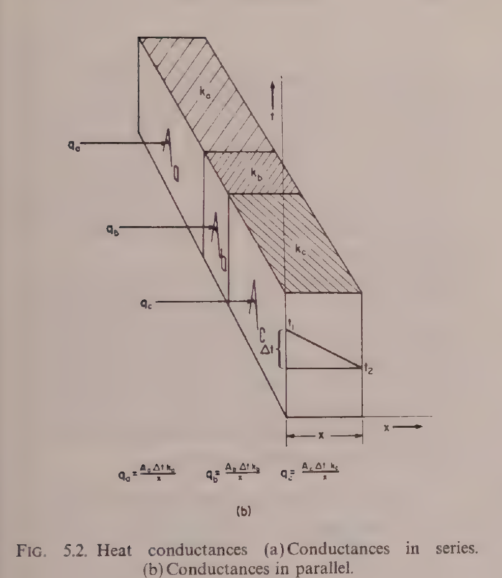
Earle Fig. 5.2(b): Heat conductances in parallel. Reproduced from Earle, Fig. 5.2(b), printed p. 49.
Practical note: when a cold room underperforms, look for the steel first: bolts, brackets, door frames and pipe supports are parallel paths that carry far more heat than their area suggests.
3.4 Thermal properties of foods: conductivity, specific heat and diffusivity
A heat transfer calculation is only as good as the properties fed into it, and foods need their own numbers. Ibarz Chapter 11 gathers them. Thermal conductivity, specific heat, density and thermal diffusivity are the four that matter, and each depends on composition and temperature.
Thermal conductivity of some foods is given in Ibarz Table 11.1. Selected values, with water content and temperature as given in the book, are:
Table 3.1: Thermal conductivity of some foods (Ibarz Table 11.1, selected values)
| Product | Water content (%) | Temperature (°C) | Thermal conductivity (J/s·m·°C) |
|---|---|---|---|
| Olive oil | - | 15 | 0.189 |
| Olive oil | - | 100 | 0.163 |
| Cod | 83 | 2.8 | 0.544 |
| Pork, perpendicular to the fibers | 75.1 | 6 | 0.488 |
| Pork, parallel to the fibers | 75.9 | 4 | 0.443 |
| Pork, fatty meat | - | 25 | 0.152 |
| Beef, lean, perpendicular to the fibers | 78.9 | 7 | 0.476 |
| Beef, lean, parallel to the fibers | 78.7 | 8 | 0.431 |
| Strawberries | - | -14 to 25 | 0.675 |
| Peas | - | 3-17 | 0.312 |
Table 3.1: Thermal conductivity of some foods, Ibarz Table 11.1, p. 329. Selected values; the full table in the book also lists soybean oil, vegetable and animal oils, sugars, lamb, veal and freeze-dried beef.
Two patterns stand out. Water content drives conductivity: lean meat at about 79% water conducts at about 0.48, while fatty meat conducts at 0.15. Direction matters too: meat conducts better across the fibers than along them, 0.488 against 0.443 for pork, because the fiber structure is not the same in both directions.
Specific heat is the energy needed to raise by 1 °C the temperature of one unit mass. For foods with a high water content above the freezing point, Siebel's equation is used:
Ĉp = 0.837 + 3.349 X_water
where Ĉp is in kJ/(kg·°C) and X_water is the mass fraction of water in the food. Charm's equation splits the food into fat, solids and water: Ĉp = 2.309 X_fat + 1.256 X_solids + 4.187 X_water. Choi and Okos give the general form as the sum over components of each component's specific heat times its mass fraction. Ibarz Table 11.4 lists measured values, including lean beef at 71.7% water with 3.433 kJ/kg·K, pasteurized whole milk at 87.0% water with 3.852 kJ/kg·K, skim milk at 90.5% water with 3.977 to 4.019 kJ/kg·K, apples raw at 84.4% water with 3.726 to 4.019 kJ/kg·K, potatoes at 79.8% water with 3.517 kJ/kg·K, and cucumbers at 96.1% water with 4.103 kJ/kg·K. The pattern is the same as for conductivity: more water means a higher specific heat, and the value for a watery food approaches that of water itself, 4.187 kJ/kg·K.
Thermal diffusivity, α, ties the three together: α = k/(ρĈp). It measures how fast a temperature change spreads through a material, rather than how much heat the material holds. Ibarz Table 11.5 gives values in units of 10⁻⁵ m²/s, including apples at 85% water and 0 to 30 °C with 1.37, strawberries pulp at 92% water and 5 °C with 1.27, avocado pulp at 24 °C with 1.24, sweet potato at 35 °C with 1.06, rising to 1.91 at 70 °C, and peas purée at 26 to 128 °C with 1.82. Diffusivity matters whenever a temperature change has to travel into the centre of a food, which is the subject of unsteady-state heat transfer and of Unit 4.
Quick check
Two foods have the same thermal conductivity, but one has twice the density and twice the specific heat of the other. Which one warms through faster, and why?
Check your answer
The lighter one, because thermal diffusivity is k divided by density times specific heat. With the same k and four times the denominator, the denser food has a quarter of the diffusivity, so a temperature change spreads four times more slowly.
3.5 Surface heat transfer: the film coefficient
So far the transfer has been through solids. In practice, heat must also pass from a fluid to a solid surface, or from a solid surface to a fluid. When heat is transferred from a fluid to a wall, some of the heat is transferred by conduction and some by convection, and the combined effect is expressed by Newton's law of cooling:
q = h_s A(t_f - t_s)
where q is the rate of heat transfer, A is the area of the surface, t_f is the temperature of the fluid, t_s is the temperature of the surface, and h_s is the surface heat transfer coefficient. The value of h_s depends on the properties of the fluid and on the nature of fluid flow near the surface. Typical values are listed in the table below.
Table 3.2: Approximate values of surface heat transfer coefficients (Earle Table 5.1)
| Fluid conditions | h_s (J m⁻² s⁻¹ °C⁻¹) |
|---|---|
| Boiling liquids | 2400-24,000 |
| Condensing liquids | 1800-18,000 |
| Still air | 6 |
| Moving air, 3 m/s | 30 |
| Liquids flowing through pipes | 1200-6000 |
Table 3.2: Approximate surface heat transfer coefficients, Earle Table 5.1, p. 62.
The range is enormous: still air transfers heat about a thousand times less well than a boiling liquid. That is why a steam jacket heats a pan far faster than a hot air oven at the same temperature, and why a still-air cold room cools food slowly.
Worked example: sugar solution in a jacketed pan (Earle Example 5.4)
Calculate the rate of heat transfer to a sugar solution in a jacketed pan from condensing steam, using the data given below. The pan contains a sugar solution of 1.4 m² area, which is maintained at 83 °C. Steam is condensing in the jacket at 200 kPa gauge, saturation temperature 134 °C, and the latent heat of the steam is 2164 kJ/kg. The heat transfer coefficient from condensing steam is 12,000 J m⁻² s⁻¹ °C⁻¹, from the sugar solution 3000 J m⁻² s⁻¹ °C⁻¹, and the wall is stainless steel 1.6 mm thick with a thermal conductivity of 21 J m⁻¹ s⁻¹ °C⁻¹.
The steam side resistance is 1/12,000, the solution side is 1/3000, and the wall resistance is 0.0016/21. Adding them: 1/U = 1/12,000 + 0.0016/21 + 1/3000, which is about 0.00049, so U is about 2030 J m⁻² s⁻¹ °C⁻¹. The temperature difference is 134 - 83 = 51 °C, so the rate of heat transfer is q = UAΔt = 2030 x 1.4 x 51 = 1.45 x 10⁵ J s⁻¹. The rate at which steam condenses is the heat rate divided by the latent heat: 1.45 x 10⁵ / 2.164 x 10⁶ = 0.067 kg s⁻¹, which is about 4 kg per minute. The solution side coefficient, 3000, is the controlling resistance: it is four times smaller than the steam side coefficient, so it dominates the sum.
Diagram: Sugar solution in a jacketed pan (Earle Example 5.4)
Steam condensing in the jacket at 134 °C
↓
Sugar solution 83 °C
Area 1.4 m²
↓
Heat rate q = 1.45 x 10⁵ J s⁻¹; steam condenses 0.067 kg s⁻¹
Diagram for Earle Example 5.4: condensing steam heats the sugar solution in the jacketed pan.
Practical note: if the soup in a jacketed pan is heating too slowly, stirring helps more than raising the steam pressure, because the liquid side film is usually the bottleneck.
3.6 The overall coefficient U and the controlling resistance
When heat passes from one fluid through a solid wall to another fluid, all the resistances are in series, and the general equation is:
1/U = 1/h₁ + x₁/k₁ + x₂/k₂ + ... + 1/h₂
where h₁ and h₂ are the surface coefficients on the two sides and the middle terms are the wall resistances. The value of U is the overall heat transfer coefficient. It depends on the nature of the fluid on both sides, on the wall material and thickness, and on the fluid velocities. When one of the surface coefficients is very large, as with condensing steam, its resistance is small and it does not control the overall coefficient. When one coefficient is much smaller than the others, it controls the overall coefficient, and improving the other resistances makes little difference. That is the single most useful insight in heat exchanger design: find the controlling resistance and attack it.
Worked example: a cold store wall with surface films (Earle Example 5.11)
The wall of a cold store is the same as in Example 5.2, brick 11 cm, concrete 7.5 cm, cork 10 cm, but now the surface coefficients are included. The outside air is moving at 6.7 m/s and the inside air at 0.61 m/s. Radiation coefficients are 6.25 J m⁻² s⁻¹ °C⁻¹ outside and 1.7 inside. The outside convection coefficient is 34, so the combined outside coefficient is 40 J m⁻² s⁻¹ °C⁻¹. The inside convection coefficient is 8.1, so the combined inside coefficient is 9.8 J m⁻² s⁻¹ °C⁻¹. The wall conductance is 0.38, as before, so 1/U = 1/40 + 1/0.38 + 1/9.8 = 2.76, which gives U = 0.36 J m⁻² s⁻¹ °C⁻¹. The heat flow is only slightly less than the 0.38 found without the films, because the cork resistance of 2.33 still dominates. The surface films matter most when the wall itself is a poor insulator, not when it is a good one.
Earle Fig. 5.2(a): Heat conductances in series, the same composite wall as in Example 5.2. Reproduced from Earle, Fig. 5.2(a), printed p. 49.
Worked example: brick against aluminium (Earle Example 5.12)
Compare the overall coefficients of two walls, one of 10 cm brick with a thermal conductivity of 0.7 J m⁻¹ s⁻¹ °C⁻¹ and one of 1.3 mm aluminium with a thermal conductivity of 208 J m⁻¹ s⁻¹ °C⁻¹. The surface coefficients are 9.9 and 40 J m⁻² s⁻¹ °C⁻¹. For the brick, 1/U = 1/9.9 + 0.10/0.7 + 1/40, which gives U = 3.7 J m⁻² s⁻¹ °C⁻¹. For the aluminium, 1/U = 1/9.9 + 0.0013/208 + 1/40, which gives U = 7.7 J m⁻² s⁻¹ °C⁻¹. The aluminium wall is only about twice as good as the brick wall, even though aluminium conducts heat about 300 times better than brick. The wall resistance is negligible in both cases, and the surface films control the result.
Diagram: Brick against aluminium (Earle Example 5.12)
k = 0.7 J m⁻¹ s⁻¹ °C⁻¹
U = 3.7 J m⁻² s⁻¹ °C⁻¹
Surface coefficients 9.9 and 40 J m⁻² s⁻¹ °C⁻¹ on the two sides
k = 208 J m⁻¹ s⁻¹ °C⁻¹
U = 7.7 J m⁻² s⁻¹ °C⁻¹
The surface films control the result in both cases
Diagram for Earle Example 5.12: a brick wall and an aluminium wall with the same surface films.
Quick check
A heat exchanger has a steam side coefficient of 12,000 and a liquid side coefficient of 300. You double the steam side coefficient to 24,000. Does the overall coefficient roughly double, or barely change?
Check your answer
Barely change. The liquid side resistance, 1/300, is forty times the steam side resistance, 1/12,000, so it controls the sum. Doubling the steam side changes the total resistance by a tiny amount.
3.7 Unsteady-state heat transfer: heating and cooling through
So far the temperatures have been steady. In food processing, temperatures change with time: a can heats up in a retort, a loaf cools on a rack, a sausage heats through in a smokehouse. That is unsteady-state heat transfer, and the temperature inside the food is not uniform. The outside heats first, and the heat then travels inward by conduction, at a rate set by the thermal diffusivity.
The method used in practice is the Gurney-Lurie charts, also called Heisler charts. For a slab, a cylinder and a sphere, the charts relate the temperature at a point inside the solid to two dimensionless groups: the Fourier number, Fo = kθ/(ρĈp r²), which is a dimensionless time, and the Biot number, Bi = h_s r/k, which compares the surface resistance with the internal resistance. When the Biot number is small, the surface resistance controls and the temperature inside the food is nearly uniform. When the Biot number is large, the internal conduction controls and a steep temperature gradient forms inside the food.
Earle works through the case of a sausage, a cylinder, heated in water, using the Gurney-Lurie charts with the food properties and the surface coefficient, to find how long it takes for the centre to reach a given temperature. The numbers in the printed scan of that example are too garbled to quote reliably, so the worked calculation is not reproduced here, and that limitation is recorded plainly: the method, the charts and the dimensionless groups are as the book gives them, but the worked numbers for Earle Example 5.5 could not be verified from the available scan.
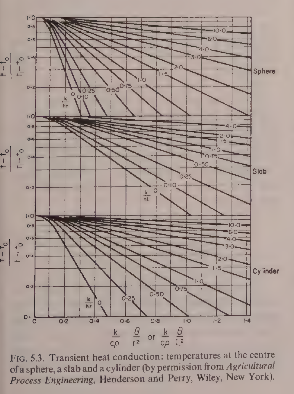
Earle Fig. 5.3: Transient heat conduction, temperatures at the centre of a sphere, a slab and a cylinder. The working charts for Earle Example 5.5. Reproduced from Earle, Fig. 5.3, printed p. 53.
The same unsteady-state idea returns in Unit 4, where the heat penetration curve of a can is the practical form of the same physics, with the centre temperature of the can tracked against time in the retort.
3.8 Radiation: heat that needs no medium
Radiation is the transfer of heat energy by electromagnetic waves. Unlike conduction and convection, it needs no medium: it crosses empty space, and it travels at the speed of light. The Stefan-Boltzmann law gives the rate at which a black body radiates heat:
q = σAT⁴
where q is the rate of heat transfer, σ is the Stefan-Boltzmann constant, A is the area of the radiating surface, and T is the absolute temperature in Kelvin. The value of σ in Earle is 5.73 x 10⁻⁸ J m⁻² s⁻¹ K⁻⁴. Real surfaces are not black bodies, and their radiation is reduced by the emissivity ε, a factor between 0 and 1, so q = εσAT⁴. Dull black surfaces have an emissivity of about 1, paper, painted metal, wood and most food surfaces about 0.9, rough unpolished metals 0.7 to 0.25, and polished metals about or below 0.05. That is why a polished steel surface stays cool in radiant heat while a blackened surface heats up.
In practice, radiation is rarely the only mechanism. A body in a room exchanges heat by radiation with the walls, and by convection with the air, at the same time. The two can be combined by defining a radiation coefficient, h_r, in the same form as a surface coefficient, so that the radiation rate is h_r A Δt, and the total coefficient is the sum of the convection and radiation coefficients. Earle uses that approach in the cold store example above, where the radiation coefficients of 6.25 outside and 1.7 inside were added to the convection coefficients.
Ibarz Chapter 14 covers the radiation laws in more depth: Planck's law for the spectrum of emitted radiation, Wien's displacement law for the wavelength of maximum emission, the Stefan-Boltzmann law for the total, and the view factor, which is the fraction of radiation leaving one surface that strikes another. The view factor matters whenever the geometry is not simple, for example a loaf on a conveyor under a bank of heaters.
Practical note: in a bakery oven, the elements glow at a high temperature and the fourth power in the Stefan-Boltzmann law makes radiation the dominant mechanism at the top of the loaf, which is why the crust browns and sets long before the crumb is done.
3.9 Convection: natural, forced, and the dimensionless groups
Convection is heat transfer by the movement of groups of molecules in a fluid. In natural convection the movement is caused by density changes: hot fluid rises, cold fluid sinks. In forced convection the fluid is moved by a pump, a fan or a stirrer. The surface coefficient h_s is the quantity that captures convection, and it is found from correlations built on dimensionless groups.
The Prandtl number, Pr = Ĉp μ/k, compares the momentum diffusivity of the fluid with its thermal diffusivity. It depends only on the fluid properties. The Nusselt number, Nu = h_s D/k, is the dimensionless form of the surface coefficient itself, for a characteristic length D. The Reynolds number, Re = Dvρ/μ, already met in Unit 2, describes the flow. A typical forced convection correlation has the form Nu = a Re^b Pr^c, with the constants depending on the geometry and the flow regime. For natural convection, the Grashof number, which contains the buoyancy force from density differences, takes the place of the Reynolds number.
Worked example: a sausage cooled in water (Earle Example 5.8)
A sausage 7.5 cm in diameter, at 74 °C, is cooled in water at 24 °C. The film temperature is (74 + 24)/2 = 49 °C, and at that temperature the water properties give a surface coefficient of 1904 J m⁻² s⁻¹ °C⁻¹, using the natural convection correlation for a horizontal cylinder. The heat transfer rate per unit area is then h_s Δt = 1904 x (74 - 24) = 95,200 J m⁻² s⁻¹. The high value, compared with still air at 6, shows what a liquid film can do.
Diagram: A sausage cooled in water (Earle Example 5.8)
Sausage 7.5 cm diameter at 74 °C
↓
Film temperature 49 °C
↓
Surface coefficient 1904 J m⁻² s⁻¹ °C⁻¹
Heat rate per unit area 95,200 J m⁻² s⁻¹
Diagram for Earle Example 5.8: a hot sausage is cooled in water at 24 °C.
Worked example: vegetable puree over a flat plate (Earle Example 5.9)
A vegetable puree flows at 3 m/min over a flat plate 0.9 m long and 0.6 m wide, held at 104 °C. The puree has a density of 1040 kg/m³, a specific heat of 3980 J kg⁻¹ °C⁻¹, a viscosity of 0.002 N s m⁻² and a thermal conductivity of 0.52 J m⁻¹ s⁻¹ °C⁻¹. The Reynolds number is 2.34 x 10⁴, so the flow is turbulent, and the Prandtl number is 15.3. The correlation then gives the Nusselt number and the surface coefficient. The final value of h_s in the printed scan is too garbled to quote reliably, so it is not reproduced here; the inputs and the two dimensionless numbers are as the book gives them.
Diagram: Vegetable puree over a flat plate (Earle Example 5.9)
Vegetable puree flows at 3 m per minute
↓
Held at 104 °C
↓
Reynolds number 2.34 x 10⁴, turbulent; Prandtl number 15.3
Diagram for Earle Example 5.9: puree flows over a flat plate held at 104 °C.
Worked example: heat loss from a cooking vessel by a draught (Earle Example 5.10)
A cooking vessel is exposed to a draught of air at 61 m/min. The surface coefficient from the book's correlation is about 9.7 J m⁻² s⁻¹ °C⁻¹. With an area of 3.4 m² and a temperature difference of 32 °C, the heat loss is about 9.7 x 3.4 x 32, which is about 1.1 x 10³ J s⁻¹. The draught matters: still air would give a coefficient of about 6, and a strong draught raises it well above that.
Diagram: Heat loss from a cooking vessel by a draught (Earle Example 5.10)
Draught of air at 61 m per minute
↓
Area 3.4 m²
Temperature difference 32 °C
↓
Surface coefficient about 9.7 J m⁻² s⁻¹ °C⁻¹
Heat loss about 1.1 x 10³ J s⁻¹
Diagram for Earle Example 5.10: a draught over the vessel raises the heat loss.
Quick check
You are cooling a hot liquid in a pipe. Would you rather increase the flow velocity or increase the pipe length to improve the heat transfer coefficient?
Check your answer
Increase the flow velocity. The surface coefficient rises with velocity through the Reynolds number, while length alone does not change the coefficient, only the area.
3.10 Heat exchangers: the machines that move heat
A heat exchanger is a device that transfers heat from one fluid to another without the two mixing, through a solid wall. The wall is usually thin metal, and the overall coefficient U is the key number. The heat transferred is:
q = UA Δt_m
where A is the heat transfer area and Δt_m is the mean temperature difference between the two fluids. The mean temperature difference is not the arithmetic mean, because the temperature difference changes along the exchanger. For two fluids exchanging heat, the logarithmic mean temperature difference is:
Δt_m = (Δt₁ - Δt₂)/ln(Δt₁/Δt₂)
where Δt₁ and Δt₂ are the temperature differences at the two ends of the exchanger.
3.10.1 Counterflow and parallel flow
The two fluids can flow in the same direction, parallel flow, or in opposite directions, counterflow. The figure below shows the temperature patterns for both. In counterflow, the temperature difference is more uniform along the exchanger, and the cold fluid can leave hotter than the hot fluid leaves. In parallel flow it cannot. For the same inlet and outlet temperatures, counterflow gives a larger logarithmic mean temperature difference, and therefore needs less area. That is why counterflow is the usual choice.
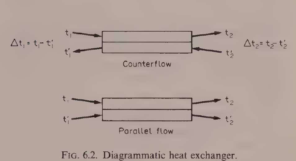
Figure 3.2: Counterflow and parallel flow in a heat exchanger. The temperature differences Δt₁ and Δt₂ are measured at the two ends, and the logarithmic mean temperature difference is (Δt₁ - Δt₂)/ln(Δt₁/Δt₂). Reproduced from Earle, Fig. 6.2, p. 66.
3.10.2 The concentric tube exchanger
The simplest heat exchanger is the concentric tube, or double pipe: one tube inside another, one fluid in the inner tube and the other in the annulus. Ibarz Figure 13.3 shows it in both arrangements.
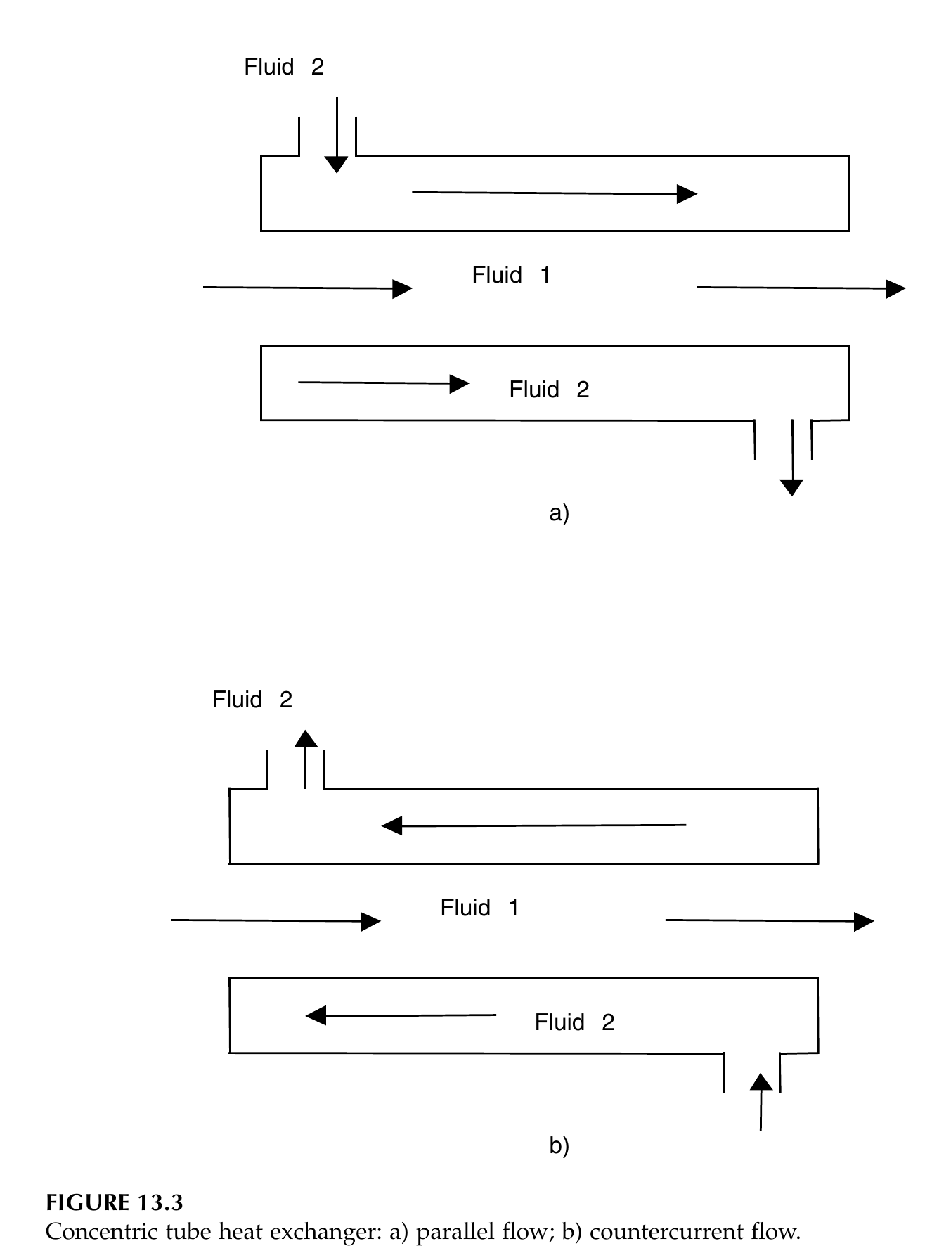
Figure 3.3: Concentric tube heat exchanger: (a) parallel flow; (b) countercurrent flow. Reproduced from Ibarz, Fig. 13.3, p. 379.
Worked example: a counterflow brine cooler (Earle Example 6.2)
In a counterflow heat exchanger, water is being chilled by a brine solution. The brine is flowing at the rate of 1.8 kg/s and its specific heat is 3.38 kJ kg⁻¹ °C⁻¹. The water is flowing at the rate of 1.05 kg/s and its specific heat is 4.18 kJ kg⁻¹ °C⁻¹. The brine enters at -8 °C and leaves at 10 °C, and the water enters at 32 °C. The exchanger has an area of 55 m². Calculate the water outlet temperature and the overall heat transfer coefficient.
The heat lost by the water equals the heat gained by the brine: 1.8 x 3.38 x (10 - (-8)) = 109.5 kJ/s. For the water, 109.5 = 1.05 x 4.18 x (32 - t_w1), so (32 - t_w1) = 109.5/(1.05 x 4.18) = 25, giving t_w1 = 7 °C. The temperature differences at the two ends are Δt₁ = 32 - 10 = 22 °C and Δt₂ = 7 - (-8) = 15 °C. The logarithmic mean temperature difference is Δt_m = (22 - 15)/ln(22/15) = 18.3 °C. The overall coefficient is U = q/(A Δt_m) = 109.5/(55 x 18.3) = 0.11 kJ m⁻² s⁻¹ °C⁻¹, which is 110 J m⁻² s⁻¹ °C⁻¹.
3.10.3 Shell and tube, plate, jacketed pan, scraped surface
The concentric tube exchanger is simple but its area per unit volume is small. For larger duties, the shell and tube exchanger is used: a bundle of tubes inside a shell, one fluid in the tubes and the other in the shell, with baffles to direct the shell side fluid across the tubes. The approach temperature, the difference between the outlet temperatures of the two fluids, can be as small as 1 °C in a shell and tube exchanger, against several degrees in simpler types, because the large area and the baffled flow make the heat transfer efficient.
The plate heat exchanger packs thin corrugated plates together, with hot and cold fluids flowing in alternate channels. The corrugations break up the flow and give high coefficients in a very small volume. Ibarz Figure 13.13 shows the construction.
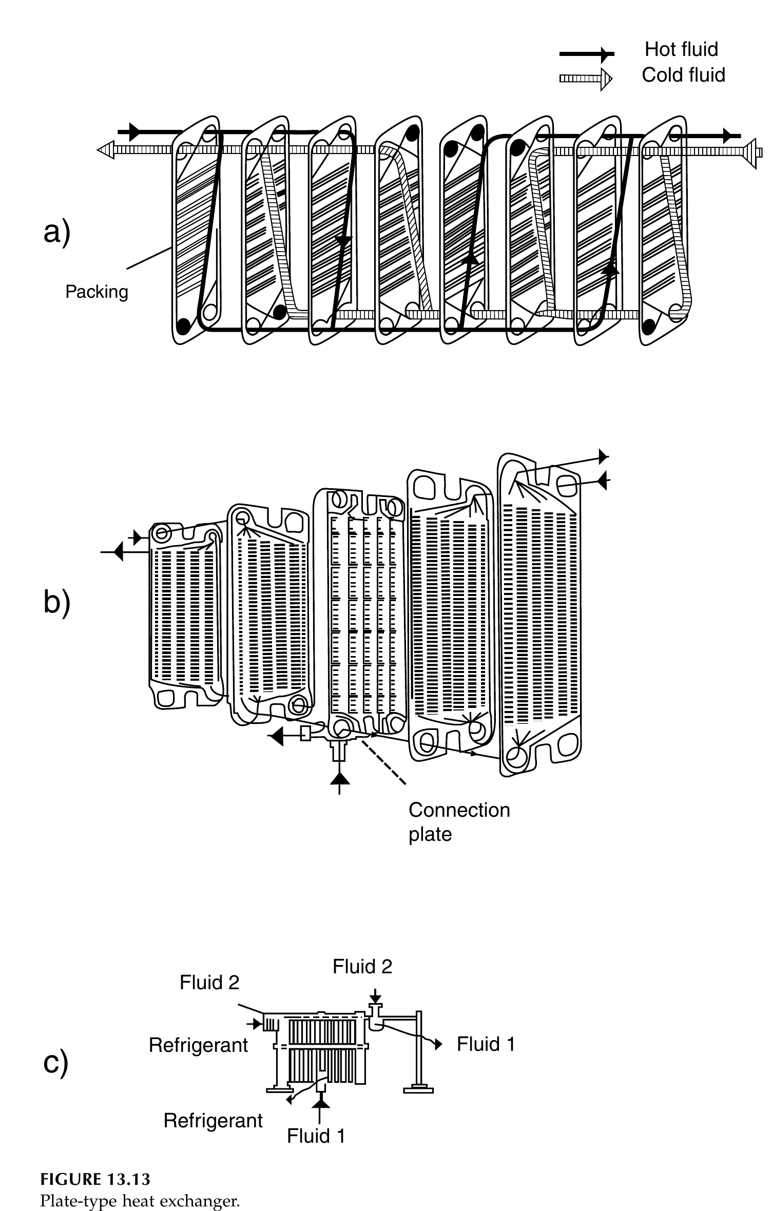
Figure 3.4: Plate-type heat exchanger: (a) plates with packing, (b) plates in exploded view, (c) plate pack with connection plate showing Fluid 1, Fluid 2 and Refrigerant connections. Reproduced from Ibarz, Fig. 13.13, p. 398.
The jacketed pan is the oldest heat exchanger in food processing: a vessel with a jacket around it, steam or hot water in the jacket, the food inside, and usually a stirrer. Earle Table 6.1 gives overall coefficients for jacketed pans, in J m⁻² s⁻¹ °C⁻¹: steam with a thin liquid in a cast iron pan, 1800; steam with a thick liquid, 900; steam with a paste in a stainless steel pan, 300; steam with boiling water in a copper pan, 1800. The coefficient falls as the food gets thicker, because the liquid side film controls, which is why a paste heats slowly even in a steam jacket.
Worked example: pea soup in a jacketed pan (Earle Examples 6.3 and 6.4)
50 kg of pea soup at 18 °C is heated in a jacketed pan by steam at 100 kPa gauge, saturation temperature 120 °C, latent heat 2202 kJ/kg. The overall coefficient is 300 J m⁻² s⁻¹ °C⁻¹ and the area is 1 m². The specific heat of the soup is 3.95 kJ kg⁻¹ °C⁻¹. Calculate the steam consumption at the start and the time needed to reach 90 °C.
At the start, the temperature difference is 120 - 18 = 102 °C, so q = UAΔt = 300 x 1 x 102 = 3.06 x 10⁴ J s⁻¹. The steam rate is q divided by the latent heat: 3.06 x 10⁴ / 2.202 x 10⁶ = 0.0139 kg s⁻¹, which is 50 kg per hour. As the soup warms, the temperature difference falls and the rate of heat transfer falls, so the time is found by integrating. The result is 803 s, which is 13.4 minutes to reach 90 °C.
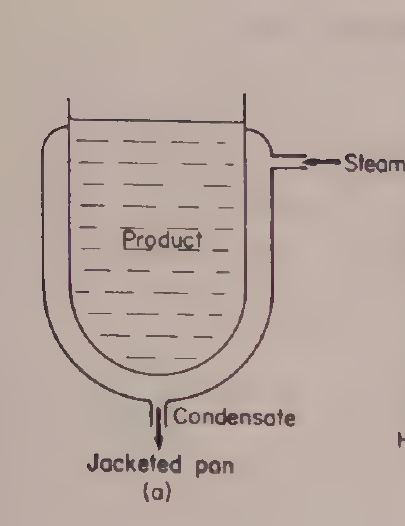
Earle Fig. 6.3(a): Jacketed pan. Reproduced from Earle, Fig. 6.3(a), printed p. 67.
The scraped surface heat exchanger is built for the foods that defeat the others: thick pastes, sticky products and foods that burn onto a hot wall. A rotor with scraper blades turns inside a cylinder, continuously scraping the product off the heated wall and mixing it. It is the exchanger of choice for products such as tomato paste, peanut butter and ice cream mix, where a plate exchanger would foul and a jacketed pan would scorch.
Quick check
You need to cool a thin juice quickly with a small temperature approach. Which exchanger type do you pick, and why?
Check your answer
A plate heat exchanger. The thin plates and corrugated channels give high coefficients and a large area in a small volume, and the approach temperature can be as small as about 1 °C.
3.11 Fouling: the dirt factor
In service, heat transfer surfaces foul. Milk stone, scale, burnt-on product and corrosion build up a layer on the wall, and that layer adds a resistance. The fouled overall coefficient U_F is related to the clean coefficient U by:
1/U_F = 1/U + R_h + R_c
where R_h and R_c are the dirt factors, or fouling resistances, on the hot and cold sides. Ibarz Table 13.1 gives dirt factors in m² °C/kW, including distilled water 0.09, sea water 0.09, river water 0.21, boiler water 0.26, very hard water 0.58, brine 0.264, organic liquids 0.176, fuel oil 1.056, tars 1.76, steam of good quality 0.052, steam of bad quality 0.09, air 0.26 to 0.53, and solvents vapour 0.14. A dirt factor of 1.056 for fuel oil means that a fuel oil film alone adds as much resistance as a clean coefficient of about 950 W/m²·°C, which is a large penalty.
The practical consequence is that heat exchangers are designed with a fouling allowance: the area is sized for the fouled condition, not the clean one. And the cleaning schedule is part of the design: a plate pasteurizer that is not cleaned on schedule will steadily lose capacity, and the outlet temperature will drift, which is a food safety matter as well as an energy matter.
Try it yourself
- Wall resistance hunt. Take the cold store wall of Example 5.2 and replace the cork with 10 cm of brick. Recompute U and the heat flow. Then replace the brick with 10 cm of cork instead. Which change matters, and why?
- Counterflow against parallel flow. For the brine cooler of Example 6.2, keep the same four temperatures but swap the flow arrangement to parallel. Work out the two end temperature differences and the logarithmic mean. How much more area would the parallel flow exchanger need for the same duty?
- Fouling check. A clean exchanger has U = 1000 J m⁻² s⁻¹ °C⁻¹. Add a dirt factor of 0.176 m² °C/kW on one side, the value for organic liquids. What is the fouled U, and by what percentage has the capacity fallen?
- Draw the temperature profile. Sketch the temperature of the hot and cold fluids along the length of a counterflow exchanger, and then along a parallel flow exchanger. Mark where the temperature difference is largest and smallest in each case.
Key ideas to carry forward
- Heat transfer rate equals driving force divided by resistance, and the driving force is the temperature difference.
- Conduction follows Fourier's law, q = kAΔt/x. Thermal conductivity is a property of the material; conductance is k/x for a real thickness.
- Resistances in series add. In a composite wall, the largest resistance controls the result.
- Resistances in parallel add as conductances. A small area of a good conductor, such as a steel bolt, can carry most of the heat.
- The overall coefficient U combines the two surface films and the wall. The smallest surface coefficient usually controls.
- Unsteady-state heat transfer is governed by thermal diffusivity, α = k/(ρĈp), and described by the Fourier and Biot numbers.
- Radiation follows the Stefan-Boltzmann law, q = εσAT⁴, and the emissivity of the surface decides how much it radiates.
- Convection correlations use the Reynolds, Prandtl and Nusselt numbers.
- In a heat exchanger, the logarithmic mean temperature difference is the correct mean, and counterflow gives a larger mean than parallel flow for the same end temperatures.
- Fouling adds a resistance. Design for the fouled condition and clean on schedule.
Glossary
Thermal conductivity (k)
A property of a material that says how well it conducts heat. High for metals, low for insulators. Example: copper conducts heat far better than cork, so a copper pan heats evenly and a cork slab insulates a cold store.
Thermal conductance (C)
The heat that passes in unit time through unit area of a specified thickness of material under unit temperature difference. C = k/x. Example: a 10 cm cork slab has a conductance of 0.43 J m⁻² s⁻¹ °C⁻¹, while a 20 cm slab has half that.
Overall heat transfer coefficient (U)
One number that combines the two surface films and the wall resistance into a single coefficient, so that q = UAΔt. Example: a jacketed pan with steam on one side and thick soup on the other has U of about 300 J m⁻² s⁻¹ °C⁻¹.
Surface heat transfer coefficient (h_s)
The coefficient that describes heat transfer between a fluid and a solid surface, combining conduction and convection in the fluid film. Example: condensing steam has h_s of about 12,000, still air about 6 J m⁻² s⁻¹ °C⁻¹.
Specific heat (Ĉp)
The energy needed to raise one kilogram of a material by 1 °C. Example: water needs 4.187 kJ/kg·°C, so a watery food such as cucumber needs more energy to heat than a fatty food.
Thermal diffusivity (α)
How fast a temperature change spreads through a material, equal to k divided by density times specific heat. Example: a food with high diffusivity warms through to the centre faster than one with low diffusivity.
Fourier number (Fo)
A dimensionless time used in unsteady-state heat transfer. Example: a large Fourier number means the heat has had time to travel deep into the food.
Biot number (Bi)
A dimensionless number comparing the surface resistance with the internal conduction resistance. Example: a small Biot number means the food temperature is nearly uniform inside, and the surface film controls.
Logarithmic mean temperature difference (LMTD)
The correct mean temperature difference to use in a heat exchanger, because the difference changes along the length. Example: for end differences of 22 °C and 15 °C, the logarithmic mean is 18.3 °C, not the arithmetic mean of 18.5 °C.
Counterflow
An arrangement in which the two fluids in a heat exchanger flow in opposite directions. Example: a counterflow brine cooler lets the water leave colder than the brine leaves, which parallel flow cannot do.
Dirt factor (fouling resistance)
An extra thermal resistance caused by deposits such as scale or burnt-on product on a heat transfer surface. Example: a fuel oil film has a dirt factor of 1.056 m² °C/kW, which cuts the capacity of an exchanger badly if it is not cleaned.
Emissivity (ε)
A number from 0 to 1 that says how well a surface radiates heat compared with a perfect black body. Example: a dull black surface radiates almost like a black body, while polished metal radiates very little.
Natural convection
Heat transfer by fluid movement caused by density changes, with hot fluid rising and cold fluid sinking. Example: a pan of soup heated from below circulates by natural convection without a stirrer.
Forced convection
Heat transfer by fluid movement caused by a pump, fan or stirrer. Example: a stirred jacketed pan heats faster than an unstirred one because the stirrer forces the soup past the wall.
References
- Earle, R. L. Unit Operations in Food Processing. 2nd edition. Pergamon Press. Chapters 5 and 6.
- Ibarz, Albert, and Barbosa-Cánovas, Gustavo V. Unit Operations in Food Engineering. CRC Press, 2003. Chapters 11, 12, 13 and 14.
- Brennan, J. G., Butters, J. R., Cowell, N. D., and Lilly, A. E. V. Food Engineering Operations. 3rd edition. Elsevier Applied Science. Chapters on heat transfer.
- Gould, Wilbur A. Unit Operations for the Food Industries. CTI Publications. Chapters on heating and heat exchangers.
- Heldman, D. R., and Singh, R. P. Food Process Engineering. 2nd edition. AVI Publishing. Chapters on heat transfer.
Unit 4: Thermal Processing, Refrigeration and Freezing
Note
Unit 4: Thermal Processing, Refrigeration and Freezing
A can of beans sits in a retort at 121 °C, and the heat creeps in from the wall to the centre, minute by minute, while the clock counts the death of spores. A tray of peas rushes through a blast freezer, and the water inside each pea turns to ice so fast the crystals stay small and the peas stay whole. A compressor squeezes a refrigerant gas, the gas gives up its heat in a condenser, and the cold that comes back is what keeps the milk at 2 °C. Three different operations, one thread: moving heat in and out of food, on purpose, with numbers.
Questions to think about
- What is the difference between pasteurization and sterilization, in engineering terms?
- Why does microbial death follow a logarithmic law, and what does that mean for a process?
- What is an F value, and how do you add up lethality across a changing temperature?
- Why is the centre of a can the coldest point, and how do engineers measure its heating?
- What decides whether ice crystals are small or large, and why does it matter?
- How does a refrigeration plant move heat uphill, from cold to hot?
- How long does it take to freeze a slab of food, and what controls that time?
4.1 Pasteurization, sterilization and commercial sterility
Heat processing of foods is done for two reasons: to destroy microorganisms and enzymes that would spoil the food or make it unsafe, and to change the food in ways people want, such as cooking. The engineering question is always the same: how much heat, for how long, at the centre of the product, where the heating is slowest.
Pasteurization is a heat treatment that destroys all pathogenic organisms and some spoilage organisms. It does not make the food stable at room temperature: a pasteurized product is unstable unless it is refrigerated. Sterilization, in the food sense, means commercial sterilization: the destruction of substantially all microorganisms and spores capable of growing under the defined storage conditions. A commercially sterile product is stable without refrigeration. The distinction is an engineering one, about the degree of destruction required, and it is decided by the target organism, the acidity of the food, and the storage conditions.
Acidity decides which treatment is needed, because acid inhibits bacterial spores. Brennan gives the demarcation at pH 4.5: low-acid foods, with pH above 4.5, need sterilization, because the spores of the most resistant organisms can grow there. Acid foods, with pH between 4.5 and 3.7, can be made safe by pasteurization. High-acid foods, below pH 3.7, are self-preserving against bacterial growth, though a mild heat treatment may still be needed to destroy enzymes and yeasts. Acid inhibition starts at about pH 5.3, and the organism of greatest concern in low-acid canning, Clostridium botulinum, is inhibited at pH 4.5. Below pH 3.7 only fungi are likely to grow. Gould gives the dividing line between acid and low-acid foods as pH 4.6, and the two figures reflect different conventions in the two books, not a disagreement about the science: the boundary sits at about pH 4.5 to 4.6, and any product near it must be treated as low-acid.
Quick check
A tomato sauce has pH 4.2 and a can of peas has pH 6.1. Which one needs a full sterilization process, and why?
Check your answer
The peas. At pH 6.1 the food is low-acid, so bacterial spores can grow and a sterilization process is needed. At pH 4.2 the acid inhibits spore growth, so pasteurization is enough.
4.2 First-order death kinetics: D and z values
When a population of microorganisms is held at a constant lethal temperature, the number of survivors falls in a regular way. The rate of death is proportional to the number still alive:
dN/dt = -kN
where N is the number of survivors at time t and k is the death rate constant. Integrating gives N = N₀ exp(-kt), an exponential decay. The death rate constants are about 10¹⁰ min⁻¹ for vegetative forms and about 1 min⁻¹ for spores, which is why spores are the hard part of thermal processing.
Because the decay is exponential, it is more convenient to count in powers of ten. The decimal reduction time, D_T, is the time at temperature T needed to reduce the population by one log cycle, that is, to one tenth of its starting number. It is related to the rate constant by D_T = 2.303/k. The time needed to achieve a given reduction is:
t = D_T log₁₀(N₀/N)
The degree of reduction is n = log₁₀(N₀/N_F), where N_F is the final number. For Clostridium botulinum, the standard is a 12 log cycle reduction, n = 12, which is the basis of the 12D concept in low-acid canning.
The D value falls as temperature rises, and the rate of that fall is measured by the z value: the temperature increase needed to reduce D by a factor of ten. For most bacterial spores the z value is about 10 °C. That single number is what lets an engineer convert a process at one temperature into an equivalent process at another.
Ibarz Figure 15.4 shows how D_T is read from a thermal death time curve. The number of survivors N is plotted on a logarithmic scale against time, giving a straight descending line. A dashed vertical line drops from N = 1000 to the line, and the D_T arrow spans one log cycle, from 1000 down to 100. That span, in minutes, is the decimal reduction time at that temperature.
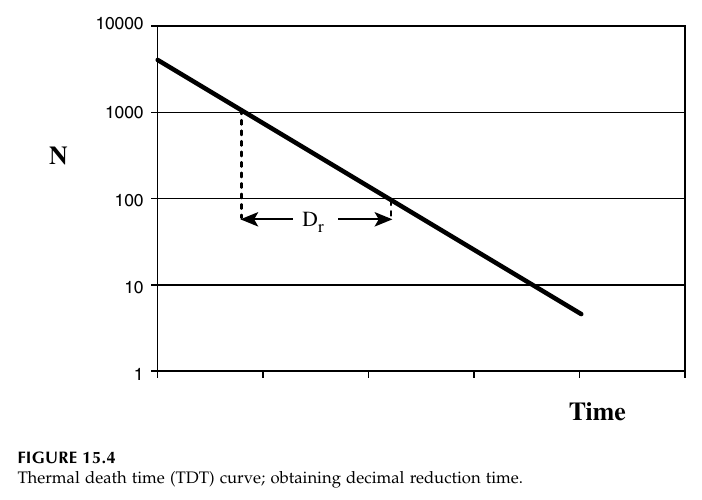
Figure 4.1: Thermal death time (TDT) curve; obtaining decimal reduction time. The number of survivors N falls in a straight line on a logarithmic scale, and D_T is the time for one log cycle of reduction. Reproduced from Ibarz, Fig. 15.4, p. 497.
The companion figure, Ibarz Figure 15.5, plots D_T itself against temperature on a logarithmic scale, giving another straight line. The z value is read from its slope: it is the temperature change that moves D_T by one log cycle. Together the two figures contain the whole kinetics of thermal death: one gives D at a temperature, the other gives how D changes with temperature.
The thermal death time for a process, F_T, is the time at temperature T needed for a given reduction: F_T = n D_T. The reference temperature for low-acid canning is 121.1 °C (250 °F), and the F value at that reference is called F₀. When a process is carried out at a different temperature, its equivalent time at the reference temperature is F_S = n D_R, where D_R is the D value at the reference temperature.
Ibarz Table 15.1 lists destruction times for thermo-sensitive microorganisms, enzymes and nutrients. Selected rows are:
Table 4.1: Destruction and thermal degradation times (Ibarz Table 15.1, selected values)
| Organism or component | Temperature (°C) | D_T (min) | F_R (min) | z (°C) | n |
|---|---|---|---|---|---|
| B. stearothermophilus (low acid, pH above 4.6) | 121 | 4-5 | 15 | 9.5-10 | 5 |
| C. botulinum (low acid, pH above 4.6) | 121 | 0.1-0.3 | 2.5-3 | 10 | 12 |
| C. sporogenes (low acid, pH above 4.6) | 121 | 0.1-1.5 | 5 | 10 | 5 |
| B. coagulans (acid, pH 4-4.6) | 121 | 0.01-0.07 | - | - | - |
| C. pasteurianum (acid, pH 4-4.6) | 93 | 0.1-0.5 | 1.3-10 | 8 | 5 |
| Yeasts and molds (very acid, pH below 4) | - | 5 x 10⁻⁸ | 10⁻⁶ | 5-8 | 20 |
| Peroxidase (sweet corn, green beans) | - | 1.22 | 5.1 | 11-52 | 4 |
| Vitamin B1 (spinach, green beans) | - | 140 | 5.6 | 25 | 0.04 |
| Chlorophyll a | - | 12.8 | 0.50 | 51-87 | 0.04 |
| Chlorophyll b | - | 14.3 | 0.57 | 98-111 | 0.04 |
Table 4.1: Destruction and thermal degradation times of thermo-sensitive microorganisms, enzymes and nutrients, Ibarz Table 15.1, p. 514. Selected rows; the full table in the book also lists other organisms and enzymes.
The table carries a lesson that shapes all of thermal processing. The z value for spores is about 10 °C, but the z value for vitamin B1 is 25 °C and for chlorophyll it is 50 to 110 °C. That means a short, hot process kills spores far more effectively, relative to the damage it does to nutrients and colour, than a long, cool process. High temperature, short time is not just a slogan: it follows directly from the different z values.
Quick check
A process gives a 6 log reduction of an organism with D = 0.5 min. How long must it run at that temperature?
Check your answer
t = n D_T = 6 x 0.5 = 3 minutes.
4.3 Lethality: adding up the F value across a real process
In a real can, the temperature is not constant. It rises during heating, holds near the retort temperature, and falls during cooling, and lethality accumulates during all three stages. The F value of a process is the sum over the whole temperature history, converting each minute at each temperature into its equivalent at the reference temperature of 121 °C:
F = θ₁ x 10^-(121-t₁)/z + θ₂ x 10^-(121-t₂)/z + ...
where θ is the time spent at temperature t, and z is 10 °C for Clostridium botulinum. A minute at 111 °C counts as 10^-1, which is one tenth of a minute at 121 °C. A minute at 101 °C counts as one hundredth. The arithmetic is simple, but it must be done at the coldest point in the can, because that is where the least lethality accumulates.
Worked example: can processing (Earle Example 6.5)
A can is processed in a retort, and the temperature at the centre of the can is recorded against time. The required F value for Clostridium botulinum is 2.8 minutes at 121 °C, with z = 10 °C. The temperature history is broken into steps, and the lethality of each step is calculated. The table below gives the steps.
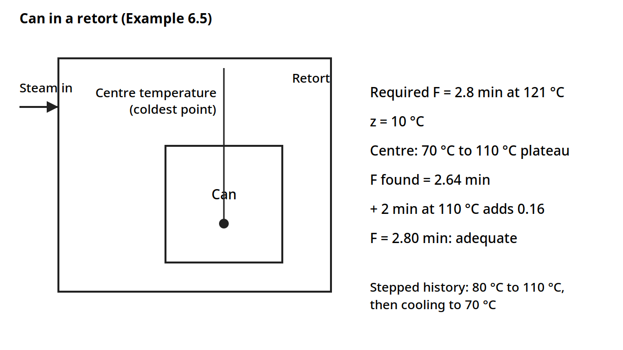
Diagram for Worked example: can processing (Earle Example 6.5). A can in a retort, with the temperature measured at the centre, the coldest point. The required F value is 2.8 minutes at 121 °C with z = 10 °C; the stepped temperature history gives F = 2.64 minutes, and 2 more minutes at 110 °C adds 0.16, making 2.80. Drawn from the book's numbers.
Table 4.2: Lethality calculation for a can process (Earle Table 6.2)
| Temperature (°C) | Time θ (min) | 121 - t | 10^-(121-t)/10 | θ x 10^-(121-t)/10 |
|---|---|---|---|---|
| 80 | 11 | 41 | 7.9 x 10⁻⁵ | 0.00087 |
| 90 | 8 | 31 | 7.9 x 10⁻⁴ | 0.0063 |
| 95 | 6 | 26 | 2.5 x 10⁻³ | 0.015 |
| 100 | 10 | 21 | 7.9 x 10⁻³ | 0.079 |
| 105 | 12 | 16 | 2.5 x 10⁻² | 0.30 |
| 108 | 6 | 13 | 5.0 x 10⁻² | 0.30 |
| 109 | 8 | 12 | 6.3 x 10⁻² | 0.50 |
| 110 | 17 | 11 | 7.9 x 10⁻² | 1.34 |
| 107 | 2 | 14 | 4.0 x 10⁻² | 0.08 |
| 100 | 2 | 21 | 7.9 x 10⁻³ | 0.016 |
| 90 | 2 | 31 | 7.9 x 10⁻⁴ | 0.0016 |
| 80 | 8 | 41 | 7.9 x 10⁻⁵ | 0.0006 |
| 70 | 6 | 51 | 7.9 x 10⁻⁶ | 0.00005 |
| Total F | 2.64 | |||
Table 4.2: Lethality calculation for a can process, Earle Table 6.2, p. 83. The total F value is 2.64 minutes.
The total F value is 2.64 minutes, against a required 2.8 minutes, so the process is not quite adequate. Adding 2 minutes at 110 °C adds 2 x 10^-(121-110)/10 = 2 x 0.079 = 0.16, making 2.80, which meets the requirement. That is how a process is adjusted in practice: a small extension at the holding temperature, where lethality accumulates fastest, rather than a long extension at a low temperature, where it barely counts.
The temperature history behind the table is shown in Earle Figure 6.6: the centre temperature rises from 70 °C to a plateau at 110 °C, holds there for about 60 to 78 minutes, and then drops sharply to 70 °C at about 95 minutes as cooling begins. The stepped approximation on the rising part is the set of steps used in the table.
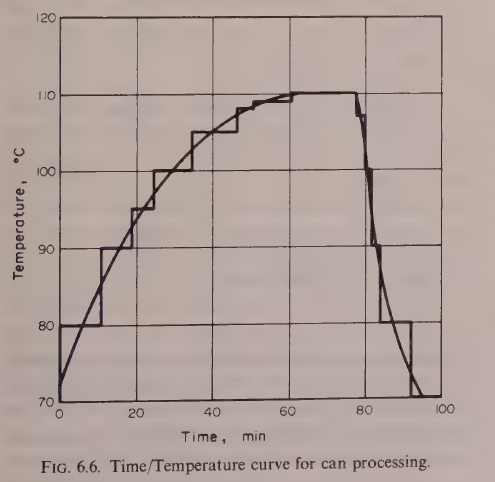
Figure 4.2: Time/temperature curve for can processing. The centre temperature rises from 70 °C to a plateau at 110 °C, holds, and then drops sharply on cooling. Reproduced from Earle, Fig. 6.6, p. 71.
Gould gives a simpler rule for low-acid sterilization: a process is considered satisfactory when the centre temperature reaches 252 °F, which is 122.4 °C, for 0.7 minute, or 42 seconds. That figure is Gould's, and it differs from the Ibarz reference temperature of 121.1 °C used in the F value calculation above. The two books use different reference conventions, and each figure must be kept with its source.
Practical note: the F value is calculated at the coldest point in the can, and the coldest point moves during the process. In a can heated by conduction, the coldest point is near the geometric centre. In a can heated by convection, the coldest point is lower, because the hot liquid rises and the cold liquid sinks. Heat penetration tests locate that point with thermocouples before the process is set.
4.4 Heat penetration: how fast does the centre warm up?
The F value calculation needs the temperature history at the centre of the can, and that history is found by heat penetration testing. A thermocouple is placed at the coldest point of the can, the can is processed in the retort, and the temperature is recorded against time. The resulting heat penetration curve is plotted on semilog paper: the vertical axis is the difference between the retort temperature and the food temperature, T_e - T, on a logarithmic scale, and the horizontal axis is time.
Ibarz Figure 15.6 shows the shape. At first the curve is bent, because the heat is still travelling in from the wall, and then it becomes a straight line. That straight part is the key to the whole method, because it is described by two numbers: f_h, the heating rate index, which is the time needed for the straight line to pass through one log cycle, and j_h, the lag factor, which measures how far the straight line, extended back to zero time, falls below the starting temperature difference. The intercept of the extended line is j_h I_h, where I_h is the initial temperature difference between the retort and the food. The process time, B, needed for the centre to reach a given temperature, is then:
B = f_h log(j_h I_h / g)
where g is the difference between the retort temperature and the final centre temperature. That equation is the formula method of Ball, and it is how a scheduled process is calculated from a heat penetration test.
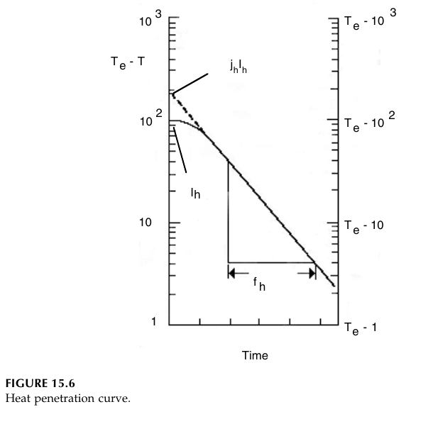
Figure 4.3: Heat penetration curve. The difference between retort temperature and food temperature, T_e - T, is plotted on a logarithmic scale against time. After an initial lag the curve is a straight line, described by the heating rate index f_h and the lag factor j_h, with intercept j_h I_h. Reproduced from Ibarz, Fig. 15.6, p. 503.
Two kinds of heating occur inside a can. In conduction heating, the food is solid or viscous, and heat travels inward by conduction, as in Unit 3. The centre heats slowly, and the temperature gradient inside the can is steep. In convection heating, the food is liquid, and the hot liquid rises and the cold liquid sinks, mixing the contents. The centre heats faster, and the temperature is more uniform. Most real foods are in between: a can of peas in brine heats partly by convection and partly by conduction, and the heating curve can show a break, called broken heating, when the mode changes during the process, for example when starch gelatinizes and the liquid thickens.
Quick check
Two cans of the same size go into the same retort. One holds a thick paste, the other holds a thin soup. Which centre heats faster, and why?
Check your answer
The soup. Its liquid circulates by convection, carrying heat to the centre, while the paste can only conduct heat inward, which is slower.
4.5 Retorts and aseptic processing
The retort is the pressure vessel in which cans are sterilized. Steam is the usual heating medium, and the retort must be vented of air before the process starts, because air in the retort lowers the temperature for a given pressure and gives an uneven heat distribution. During heating, the pressure inside the can rises as the food approaches retort temperature, and the can is under tension; during cooling, the retort pressure must be balanced with air pressure, or the cans will buckle. Batch retorts hold a fixed number of cans and run one process at a time. Continuous retorts move the cans through on a conveyor or in a rotary system, with axial rotary movement of the cans, and they are used where the volume justifies them. Non-agitating batch retorts are used extensively in spite of their slower heating, because they are simple and flexible.
Aseptic processing separates the two steps that canning combines. The food is sterilized first, in a continuous heat exchanger, and then packed in a sterilized container under sterile conditions. Because the food is heated in a thin stream rather than in a can, the heating is fast and uniform, the holding time is short, and the quality is better: less cooked flavour, less colour loss, less nutrient damage, and less energy used. The engineering problem moves from the can to the heat exchanger and the sterile filler, and the process time is calculated from the residence time distribution of the product in the holding tube, because the fastest particle through the tube gets the least treatment.
4.6 Freezing: ice, crystals and freezing time
Freezing is the removal of heat until the water in the food turns to ice. Pure water freezes at 0 °C: on cooling it subcools slightly below 0 °C, then the temperature rises back to 0 °C as ice begins to form, stays constant while all the water turns to ice, and then falls faster, because ice conducts heat better than liquid water. Foods do not behave like pure water, because as ice forms, the solutes left behind become more concentrated, and the freezing temperature falls continuously. A food does not have one freezing temperature: it has a range, and the first ice forms at the initial freezing temperature, which depends on the composition.
Table 4.3: Initial freezing temperature of some foods (Ibarz Table 16.1, selected values)
| Product | Moisture (%) | Initial freezing temperature (°C) |
|---|---|---|
| Meat | 55-70 | -1.0 to -2.2 |
| Fish | 65-81 | -0.6 to -2.0 |
| Egg | 74 | -0.5 |
| Milk | 87 | -0.5 |
| Fruits | 87-95 | -0.9 to -2.7 |
| Strawberry | - | -0.89 |
| Raspberry | - | -1.22 |
| Peach | - | -1.56 |
| Pear | - | -1.61 |
| Plum | - | -2.28 |
| Cranberry | - | -1.11 |
| Vegetables | 78-92 | -0.8 to -2.8 |
| Onion | - | -1.44 |
| Asparagus | - | -0.67 |
| Spinach | - | -0.56 |
| Carrot | - | -1.11 |
| Orange juice | - | -1.17 |
| Tomato pulp | - | -0.72 |
| Apple concentrate | 49.8 | -11.33 |
Table 4.3: Initial freezing temperature of some foods, Ibarz Table 16.1, p. 555. Selected values; the full table in the book also lists other fruits, vegetables and juices.
The rate of freezing decides the quality of the frozen food. Fast freezing gives many nucleation sites and small ice crystals, which form inside the cells and do little damage. Slow freezing gives few nucleation sites and large ice crystals, which grow between the cells, crush the tissue, and on thawing leave a soft, leaky product. That is why quick freezing is the objective of the industry, and why the freezing equipment of section 4.8 is built for speed.
Two definitions of freezing time are used. The effective freezing time is the time for the geometric centre of the food to go from its initial temperature to a given final temperature below freezing. The nominal freezing time is the time from when the surface reaches 0 °C until the centre reaches 10 °C below the initial freezing temperature. The two differ, and the definition in use must be stated whenever a freezing time is quoted.
The freezing time for a simple shape is given by Plank's equation. For an infinite slab of thickness e:
t_F = ρλ_I / (T_F - T_e) x (e²/(8k) + e/(2h))
where ρ is the density, λ_I is the latent heat of the frozen water fraction, T_F is the freezing temperature, T_e is the temperature of the cooling medium, k is the thermal conductivity of the frozen food, and h is the surface coefficient. The equation is valid only for the freezing period, and it assumes the food is initially at its freezing temperature. For a cylinder the 8 and 2 become 16 and 4, and for a sphere they become 24 and 6, with the radius as the characteristic dimension. The generalized form uses parameters P and R, given in Ibarz Table 16.2: an infinite slab has P = 1/2 and R = 1/8 with thickness e; an infinite cylinder has P = 1/4 and R = 1/16 with radius r; a sphere has P = 1/6 and R = 1/24 with radius r. The latent heat of the frozen water is λ_I = x_H λ, where x_H is the mass fraction of water that freezes and λ is the latent heat of water. The Fourier, Biot and Stefan numbers, met in Unit 3, appear in the more refined treatments, and the Cleland and Earle modification of Plank's equation improves the prediction for foods that are not initially at the freezing temperature.
The heat load of freezing is large, because the latent heat of water is large. Earle's bread freezing example in Unit 1 showed the scale: freezing a batch of bread removed a total enthalpy of 1.125 x 10⁶ kJ, at an average rate of 52 kW and a maximum rate of 104 kW. A freezing plant must be sized for that peak, not for the average.
Quick check
Two identical slabs of the same food are frozen, one in still air and one in a fast air blast. Which freezes faster, and which part of Plank's equation explains it?
Check your answer
The one in the air blast. The surface coefficient h is larger, so the term e/(2h) is smaller, and the freezing time falls. The conduction term e²/(8k) is unchanged.
4.7 Refrigeration: moving heat uphill
Refrigeration is the extraction of heat from a cold place and its rejection to a warmer place, which needs work. Gould puts it plainly: cold never moves in, heat moves out. The machine that does it is the vapour compression cycle, shown in Ibarz Figure 16.4. A refrigerant evaporates in the evaporator, taking heat from the food or the cold room. The vapour is compressed in the compressor, which raises its temperature and pressure. The hot vapour condenses in the condenser, giving up its heat to cooling water or air. The liquid then passes through the expansion valve, where its pressure and temperature fall, and returns to the evaporator.
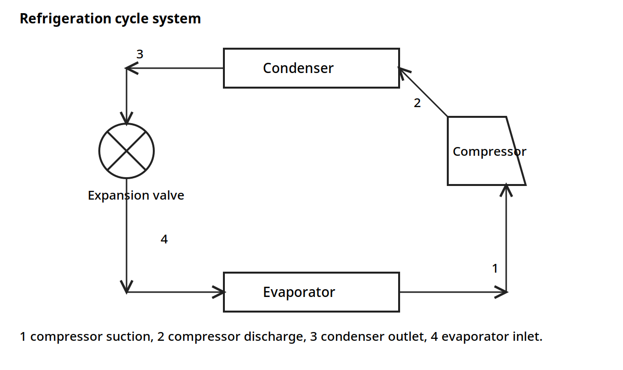
Figure 4.4: Refrigeration cycle system. The refrigerant evaporates in the evaporator, is compressed in the compressor, condenses in the condenser, and expands through the expansion valve. Reproduced from Ibarz, Fig. 16.4, p. 553, adapted from Stoecker and Jones, Refrigeration and Air Conditioning, McGraw-Hill, New York, 1982.
The compression work per unit mass of refrigerant is W_C = H₂ - H₁, where H₁ is the enthalpy at the compressor suction and H₂ is the enthalpy at the compressor discharge. The theoretical compressor power is Pow = w W_C = w(H₂ - H₁), where w is the mass flow rate of refrigerant. Those two equations, with the refrigerant tables, are the basis of refrigeration plant sizing.
Many plants need more than one temperature. A dairy, for example, may have one evaporator at -35 °C to harden ice cream and another at 2 °C to cool milk, both served by the same plant. That is a multipressure system: two evaporators at different pressures, with the vapour from the warmer evaporator compressed in stages or boosted to the level of the colder one.
The size of a refrigeration plant is often quoted in tons of refrigeration. One ton of refrigeration is the melting of one ton of ice in 24 hours, which is 288,000 BTU per 24-hour day, from 2000 lb of ice at 144 BTU per lb. It is an old unit, but it is still the unit the industry uses.
Table 4.4: Refrigerants (Ibarz Table 16.6, selected values)
| Refrigerant number | Chemical name | Formula |
|---|---|---|
| 11 | Trichlorofluoromethane | CCl₃F |
| 12 | Dichlorodifluoromethane | CCl₂F₂ |
| 13 | Chlorotrifluoromethane | CClF₃ |
| 22 | Chlorodifluoromethane | CHClF₂ |
| 40 | Chloromethyl | CH₃Cl |
| 113 | Trichlorotrifluoroethane | CCl₂FCClF₂ |
| 114 | Dichlorotetrafluoroethane | CClF₂CClF₂ |
| 50 | Methane | CH₄ |
| 170 | Ethane | C₂H₆ |
| 290 | Propane | C₃H₈ |
| 717 | Ammonia | NH₃ |
| 718 | Water | H₂O |
| 729 | Air | - |
| 744 | Carbon dioxide | CO₂ |
| 764 | Sulfur dioxide | SO₂ |
Table 4.4: Refrigerants, Ibarz Table 16.6, p. 572. Source: Stoecker and Jones, 1982. The book notes that halocarbons harm the ozone layer, that their use is limited, and that some are banned.
The book's table is given as the book gives it. Ammonia, number 717, remains the workhorse refrigerant of large food plants, because it is efficient and cheap, though it is toxic and needs careful handling. The halocarbons in the table were the common refrigerants when the book was written, and the book itself notes the ozone problem and the limits on their use.
4.8 Freezing equipment
Freezing equipment is built to remove heat fast, because fast freezing means small ice crystals and good quality. Gould classifies freezers into five types: still freezing in air; air blast or forced air freezers, generally in tunnels, but also in rooms with cold air circulating at more than 2,000 cubic feet per minute; single or double contact freezers, for packaged items; spray or fog freezers, with refrigerant sprayed over the packed or loose product; and direct or indirect immersion freezers, in which the product is immersed in the refrigerant, either packed or loose. Refrigerants vary from low pressure ammonia units to liquid nitrogen.
The plate freezer is the contact freezer: the food, usually packaged, is pressed between cold plates, and heat leaves by conduction through the plates. Horizontal plate freezers are the older form, and vertical plate freezers are a more recent development. The surface of the food and the cooling medium must be in good contact, because any air gap is an insulating layer, and the same lesson from Unit 3 applies: the largest resistance controls.
The air blast freezer is the workhorse for unpackaged foods. Cold air is blown at high speed over the product, in a tunnel or a room, and the high air velocity raises the surface coefficient. Continuous air blast freezers move the product through on a belt. The fluidized bed freezer is a form of air blast freezer for small loose pieces such as peas and berries: the air velocity is high enough to lift and suspend the pieces, so every surface is exposed to the cold air, and the pieces freeze separately instead of in a block. One of its major advantages is the ease with which the product can be handled afterwards, since the pieces stay free flowing.
Cryogenic freezing uses liquid nitrogen as the refrigerant. The product may be packaged and placed on trays, or individually quick frozen on belts and then packaged, or handled in bulk for secondary processing. The advantage of liquid nitrogen is a very rapid freezing rate and generally good preservation of quality in terms of texture, at least. The cost is high, so it is used where the quality justifies it. Frozen foods must always be kept frozen, in transport and storage below 0 °F, which is -17.8 °C, and the shelf life is restricted to time, usually not more than one year.
Quick check
You need to freeze loose peas so they stay separate and free flowing. Which freezer type do you pick, and why?
Check your answer
A fluidized bed freezer. The air lifts and suspends the peas, so every surface is exposed and the peas freeze separately instead of in a block.
Try it yourself
- Lethality addition. A can spends 5 minutes at 115 °C and 10 minutes at 110 °C, with z = 10 °C. What F value does it accumulate? How many more minutes at 110 °C would it need to reach F = 2.8?
- D value from a graph. Draw a TDT curve with D = 2 minutes. If the starting population is 10,000, how many survivors remain after 6 minutes? After 8 minutes?
- Plank in practice. A slab of food 4 cm thick is frozen in a blast freezer. If the thickness is doubled to 8 cm, what happens to the freezing time? Which term in Plank's equation grows, and by how much?
- Refrigeration load. A plant must remove 104 kW at peak, the bread freezing figure from Unit 1. Express that load in tons of refrigeration, using 1 ton = 3.517 kW. How many tons is the peak load?
- Crystal size. Freeze two identical samples of the same food, one in still air and one in liquid nitrogen. Predict which has smaller ice crystals, and say what happens to the texture of each on thawing.
Key ideas to carry forward
- Pasteurization destroys pathogens and some spoilage organisms; commercial sterilization destroys substantially all organisms and spores capable of growing under the storage conditions.
- Acidity decides the treatment: low-acid foods above about pH 4.5 need sterilization, acid foods can be pasteurized.
- Microbial death is first order: N = N₀ exp(-kt). The D value is the time for one log cycle of reduction, and the z value is the temperature rise that cuts D by ten.
- The F value adds up lethality across a changing temperature history, converted to equivalent minutes at 121 °C.
- The heat penetration curve, plotted on semilog paper, gives f_h and j_h, and the process time follows from B = f_h log(j_h I_h / g).
- Different z values for spores and for nutrients are the reason high temperature, short time processes protect quality.
- Fast freezing gives small ice crystals and good texture; slow freezing gives large crystals that damage tissue.
- Plank's equation gives the freezing time for a slab, cylinder or sphere, and it assumes the food starts at its freezing temperature.
- The vapour compression cycle moves heat from cold to hot using work: evaporation, compression, condensation and expansion.
- Freezing equipment is chosen for speed: plate, air blast, fluidized bed, immersion and cryogenic freezers each suit different products.
Glossary
Decimal reduction time (D value)
The time at a given temperature needed to reduce a microbial population by one log cycle, to one tenth of its starting number. Example: C. botulinum has a D value of 0.1 to 0.3 minutes at 121 °C.
z value
The temperature increase needed to reduce the D value by a factor of ten. Example: most bacterial spores have a z value of about 10 °C.
F value
The time at the reference temperature of 121.1 °C that gives the same lethality as the actual process. Example: a can process with F = 2.64 minutes is not quite enough when 2.8 minutes is required.
Commercial sterility
The destruction of substantially all microorganisms and spores capable of growing under the defined storage conditions, so the product is stable without refrigeration. Example: a canned bean is commercially sterile, while pasteurized milk is not.
Heat penetration curve
A plot of the difference between retort temperature and food temperature, on a logarithmic scale, against time, measured at the coldest point of the can. Example: the straight part of the curve gives f_h and j_h for the Ball formula method.
Heating rate index (f_h)
The time needed for the straight part of the heat penetration curve to pass through one log cycle. Example: a small f_h means the centre of the can heats fast.
Lag factor (j_h)
A number that measures how far the straight part of the heat penetration curve, extended back to zero time, falls below the starting temperature difference. Example: a large lag factor means the centre is slow to start warming.
Retort
A pressure vessel in which cans are sterilized with steam. Example: a batch retort holds a fixed number of cans and runs one process at a time.
Aseptic processing
Sterilizing the food first, in a continuous heat exchanger, and then packing it in a sterilized container under sterile conditions. Example: long-life milk in a carton is made by aseptic processing.
Initial freezing temperature
The temperature at which the first ice forms in a food, which falls as solutes concentrate during freezing. Example: milk starts to freeze at -0.5 °C, while apple concentrate starts at -11.33 °C.
Plank's equation
The equation that predicts the freezing time of a slab, cylinder or sphere from its size, density, latent heat, conductivity and surface coefficient. Example: doubling the thickness of a slab quadruples the conduction term in the freezing time.
Effective freezing time
The time for the geometric centre of the food to go from its initial temperature to a given final temperature below freezing. Example: a freezing time quoted without saying whether it is effective or nominal cannot be compared with another.
Refrigerant
The fluid that carries heat around a refrigeration cycle by evaporating and condensing. Example: ammonia, number 717, is the workhorse refrigerant of large food plants.
Ton of refrigeration
A unit of refrigeration capacity equal to melting one ton of ice in 24 hours, which is 288,000 BTU per 24-hour day. Example: a plant rated at 100 tons can remove about 352 kW of heat.
Fluidized bed freezer
A freezer in which cold air lifts and suspends small loose pieces, so every surface is exposed and the pieces freeze separately. Example: peas and berries are frozen in a fluidized bed so they stay free flowing.
References
- Earle, R. L. Unit Operations in Food Processing. 2nd edition. Pergamon Press. Chapter 6.
- Ibarz, Albert, and Barbosa-Cánovas, Gustavo V. Unit Operations in Food Engineering. CRC Press, 2003. Chapters 15 and 16.
- Brennan, J. G., Butters, J. R., Cowell, N. D., and Lilly, A. E. V. Food Engineering Operations. 3rd edition. Elsevier Applied Science. Chapters 10 and 13.
- Gould, Wilbur A. Unit Operations for the Food Industries. CTI Publications. Chapters 17 and 18.
- Heldman, D. R., and Singh, R. P. Food Process Engineering. 2nd edition. AVI Publishing. Chapters on thermal processing and freezing.
Unit 5: Mass Transfer and Contact-Equilibrium Separations
Note
Unit 5: Mass Transfer and Contact-Equilibrium Separations
A spoonful of sugar stirred into hot tea disappears. The sugar does not vanish: it moves, molecule by molecule, from the solid crystal into the water until the water can hold no more at that temperature. A bubble of steam rising through cream carries away a faint off flavour that no filter could catch. A column of small ceramic rings lets a gas and a liquid pass each other in opposite directions, and a gas that went in dirty comes out clean. All three are the same kind of event: matter moving from one place, or one phase, to another, driven by a difference in concentration. This unit is about that movement, and about the machines that make it useful.
Questions to think about
- What makes a component move from one phase to another, and what makes it stop?
- Why does a gas dissolve faster in cold water than in hot water?
- What happens in the thin films on each side of a gas-liquid interface?
- How does a designer decide how tall an absorption column must be?
- Why does sugar sometimes refuse to crystallize from a solution that holds too much of it?
- How can a solid pull a bitter compound out of orange juice without heating the juice?
5.1 Mass transfer: matter on the move
Every separation in this unit rests on one plain fact: when the concentration of a component is not the same everywhere, the component moves from where there is more of it to where there is less, until the concentrations even out. That movement is mass transfer. It is the third of the three transport processes, beside momentum transfer (flow) and heat transfer, and it follows the same pattern as the other two: a driving force divided by a resistance gives a rate.
In a still mixture the movement is molecular diffusion, described by Fick's law. Ibarz states it in the form used through Chapter 20:
Nᵢ = -D ∂C/∂z (20.8)
Here Nᵢ is the diffusion flux rate, C is the concentration, z is the distance or position, and D is the diffusivity. The minus sign says the flux runs downhill, from high concentration to low. The law applies at a single point, so for real equipment the book uses integrated forms of it, as Section 5.3 shows.
Diffusion is fast in gases and much slower in liquids. That single difference shapes most of the equipment in this unit: gases meet liquids over large surfaces, in thin films and small droplets, because the slow liquid side needs all the help it can get. Diffusion also explains ordinary food events: salt moving into a cucumber in brine, sugar moving out of a beet slice into hot water, an aroma compound escaping from a cut apple into the air. In each case a concentration difference is the push, and the rate depends on how steep the difference is and how easily the molecules can move through the material in their way.
Quick check
What does Fick's law say the diffusion flux is proportional to?
Check your answer
The concentration gradient, ∂C/∂z: the steeper the change of concentration with distance, the larger the flux, and the flux runs from high concentration to low.
5.2 Equilibrium: where the movement stops
Mass transfer stops when the phases in contact reach equilibrium. Earle puts the idea in one sentence that runs through the whole of his Chapter 9: the equilibrium concentrations of components often differ across the boundary between one phase and another, and those differences can be used to separate mixtures by enriching one phase relative to the other. The transfer goes on only while the actual concentration differs from the equilibrium concentration. That difference is the driving force.
Three simple laws describe equilibrium for the systems in these books.
Dalton's law. In a gas mixture the total pressure is the sum of the partial pressures, and each partial pressure is proportional to the mole fraction of that component in the vapour: pᵢ = yᵢP (Ibarz Eq. 19.1; Earle Eq. 9.3). Earle works this out for air in Example 9.2: air is reported as 79 parts nitrogen to 21 parts oxygen by volume, so the mole fractions are 0.79 nitrogen and 0.21 oxygen. With molecular weights 28 for nitrogen and 32 for oxygen, the weight fractions are 0.77 nitrogen and 0.23 oxygen, and the mean molecular weight of air is 28.8, say 29.
Raoult's law. For an ideal liquid mixture the partial pressure of a component is proportional to its mole fraction in the liquid, with the vapour pressure of the pure component as the factor: pᵢ = xᵢpᵢ° (Ibarz Eq. 19.2). The book notes that this holds in general only at high values of xᵢ, and over the whole range only for ideal solutions.
Henry's law. For a dilute solution the partial pressure is proportional to the mole fraction in the liquid, with a constant H that belongs to that gas, that liquid and that temperature: pᵢ = Hxᵢ (Ibarz Eq. 20.1; Earle Eq. 9.4). Henry's law is the workhorse of absorption design, and it is used in this unit for dilute systems where the mole fraction of the solute is below about 0.1. H changes strongly with temperature, and Ibarz gives the form log H = A + B/T, where T is the absolute temperature and A and B are constants. For a given system the equilibrium curve at a higher temperature sits above the curve at a lower temperature: warm liquid holds less gas, so gas comes out of solution when the liquid is heated, which is why a fizzy drink goes flat faster when it is warm.
Earle states the same law in the form pₐ = Hₐxₐ and notes that H has units of kPa per mole fraction. Example 9.3 uses it for carbon dioxide in water at 25°C, where H is 1.6 x 10⁵ kPa per mole fraction, with a carbon dioxide partial pressure of 200 kPa above the water. From p = Hx, x = 200/(1.6 x 10⁵) = 0.00125. Converting mole fraction to weight gives w(CO₂)/w(H₂O) = 1.25 x 10⁻³ x 44/18 = 3.1 x 10⁻³, that is 0.31% by weight. That small number is the whole story of carbonated drinks: even under pressure, water holds only a fraction of a percent of carbon dioxide, and it holds it only while the pressure stays on.
Mole fractions are the natural units here, because gas laws count molecules, not kilograms. Example 9.1 shows the conversion for a solution of 30% ethanol by weight in water. The molecular weight of ethanol, C₂H₅OH, is 46 and of water, H₂O, is 18. In 100 kg of mixture there are 30 kg of ethanol and 70 kg of water, so the mole fraction of ethanol is (30/46)/(30/46 + 70/18) = 0.144, and the mole fraction of water is (70/18)/(30/46 + 70/18) = 0.856, which is 1 - 0.144. A worker who confuses weight fraction with mole fraction in a design calculation will get the equilibrium wrong by a large factor, so the books make this conversion explicit.
Quick check
Warm water holds less dissolved gas than cold water. Which law's constant changes with temperature to describe that, and in which direction does the equilibrium curve move when temperature rises?
Check your answer
Henry's law: the constant H varies with temperature, and the equilibrium curve at a higher temperature sits above the curve at a lower temperature, so less gas stays dissolved.
Try it yourself: see equilibrium move
Pour two glasses of a carbonated drink. Leave one cold and let the other warm to room temperature, then open both. Watch which one keeps its bubbles longer and which one goes flat first. The cold glass holds more gas because its equilibrium curve sits lower. Now stir the warm glass gently: stirring does not change the equilibrium, it only helps the drink reach it faster. That is the difference between equilibrium, which sets where the system ends up, and rate, which sets how fast it gets there. Both ideas run through this unit.
5.3 The double film: what happens at the interface
When a gas meets a liquid, the transfer does not happen in the bulk of either phase. It happens across the interface, and the double film theory of Whitman (1923) gives the clearest picture of how. Ibarz presents it as the simplest model, and it is the one used through Chapter 20.
The picture is this. On each side of the interface there is a thin, still film of fluid, a laminar layer through which transfer happens only by molecular diffusion. Outside those films, in the bulk gas and the bulk liquid, mixing is good and there is no concentration gradient. At the interface itself the gas and the liquid are in equilibrium with each other. So the concentration is flat in the bulk gas, falls across the gas film, jumps at the interface to the equilibrium value, then falls across the liquid film to the flat value in the bulk liquid.
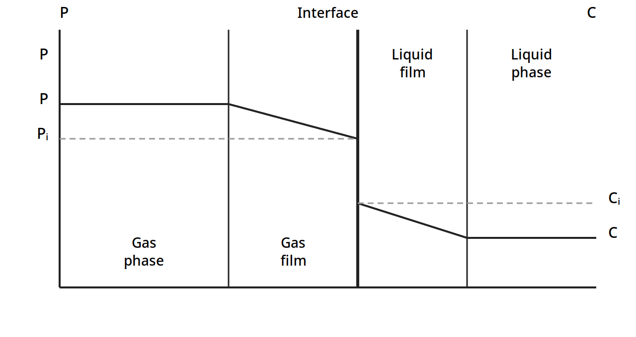
Figure 5.1: Concentration profiles in double film. The partial pressure P is flat in the bulk gas, falls across the gas film to the interface value Pᵢ, and the concentration C is flat in the bulk liquid, rising across the liquid film to the interface value Cᵢ. The gas and liquid compositions at the interface are in equilibrium. (Ibarz, Fig. 20.3, p. 728)
The flux through each film follows Fick's law in integrated form. For a component A diffusing through a stagnant gas B, Ibarz gives Nₐ = (Dv/L)(Cɢ - Cɢⁱ) (20.9), where L is the film thickness, Dv the diffusivity in the gas, Cɢ the concentration in the bulk gas and Cɢⁱ the concentration at the interface. For ideal gases this becomes Nₐ = (Dv/RTL)(P - Pᵢ) (20.10), and with the individual gas-phase coefficient kɢ = Dv/RTL (20.11), the flux is Nₐ = kɢ(P - Pᵢ) (20.12). For the liquid film, with kₗ = Dₗ/L (20.14), the flux is Nₐ = kₗ(Cᵢ - C) (20.15).
At steady state the flux through the gas film equals the flux through the liquid film, so Nₐ = kɢ(P - Pᵢ) = kₗ(Cᵢ - C) (20.16). The interface compositions Pᵢ and Cᵢ are hard to measure, so the book replaces them with overall coefficients Kɢ and Kₗ, defined against the equilibrium values: Nₐ = Kɢ(P - Pₑ) = Kₗ(Cₑ - C) (20.18), where Pₑ is the partial pressure in equilibrium with the bulk liquid concentration C, and Cₑ is the concentration in equilibrium with the bulk gas pressure P. The individual and overall coefficients are linked by 1/Kɢ = 1/kɢ + n'/kₗ and 1/Kₗ = 1/kₗ + n''/kɢ in the book's notation (Eq. 20.23), where n' and n'' are the local slopes of the equilibrium curve; when Henry's law holds, n' = n'' = H.
That pair of resistances is the practical heart of the chapter. If the gas is very soluble, the liquid film offers almost no resistance, Cᵢ is close to C, and the gas phase controls the rate, so kɢ = Kɢ. If the gas is only slightly soluble, the gas film offers almost no resistance, Pᵢ is close to P, and the liquid phase controls, so kₗ = Kₗ. A designer who knows which side controls knows where to spend effort: more gas turbulence helps only when the gas side controls, and more liquid mixing helps only when the liquid side controls. In food work the liquid side usually controls, because diffusion in liquids is slow, which is why absorption equipment works so hard to spread the liquid thin and keep it moving.
Earle gives the same idea in a single rate equation for gas absorption: dw/dθ = K_yA(y - y*), where y is the concentration in the gas, y* the concentration in equilibrium with the liquid, A the contact area and K_y an overall coefficient. The rate is the driving force (y - y*) times a coefficient times the area. Everything in absorption design is a way of making one of those three bigger: a larger driving force, a larger coefficient, or more area.
Quick check
A gas is very soluble in the liquid it is being absorbed into. Which phase controls the rate, and what does that mean for the two film coefficients?
Check your answer
The gas phase controls. The liquid film offers almost no resistance, so the interface liquid concentration is close to the bulk liquid concentration, and the gas coefficient equals the overall gas coefficient, kₗ = Kₗ.
5.4 Absorption columns: packing, flooding and height
Absorption is usually carried out in a column, with gas rising and liquid falling in countercurrent flow, because that arrangement keeps the largest concentration difference between the phases along the whole column. Ibarz describes two kinds of column: the packed column, in which transfer happens continuously along a bed of inert packing, and the plate column, in which transfer happens stage by stage on plates.
The packed column
A packed column is a tower filled with a bed of inert solid pieces called packing. Liquid enters at the top through a distributor that spreads it evenly over the packing, and gas enters at the bottom and rises through the gaps. The packing gives a large contact surface between the phases. Ibarz lists the design steps in order: selection of the solvent, obtaining equilibrium data, mass balance, enthalpy balance, selection of packing, calculation of the column diameter, calculation of packing height, and calculation of pressure drop.
The ideal solvent is not volatile, not corrosive, not viscous, not foaming, stable, not flammable, and does not dissolve the solute without limit. No real solvent meets every point, so the choice is a compromise, with liquids that dissolve the solute well preferred, and, for physical absorption, the cheapest and least corrosive solvent chosen.
The mass balance is written in molar ratios, Y for the gas and X for the liquid, with G' the inert gas molar flow and L' the solvent molar flow. The solute lost by the gas equals the solute gained by the liquid: G'(Y₁ - Y₂) = L'(X₁ - X₂) (20.25). That balance is a straight line on the Y-X diagram, the operating line, with slope L'/G', joining the bottom conditions (X₁, Y₁) to the top conditions (X₂, Y₂). For absorption the equilibrium curve lies below the operating line; for desorption, or stripping, the operating line lies below the equilibrium curve. If the solvent flow is reduced until the operating line just touches the equilibrium curve, the outlet liquid is in equilibrium with the inlet gas, and the ratio (L'/G') is at its minimum (Eq. 20.27). Reaching that point would need a tower of infinite height, so in practice the book uses a ratio 25% above the minimum: L'/G' = 1.25 (L'/G')min.
Packing: what it is and what it does
Packing must be chemically inert to the fluids, strong enough without excessive weight, open enough to let both streams pass without excessive liquid holdup or pressure drop, good at bringing the phases into contact, and relatively cheap. Ibarz classifies the common types as rings and saddles. Raschig rings are the simplest and most common, a short piece of tube with height equal to its diameter. Lessing rings add a transverse partition wall to increase contact surface, with a maximum size of 6 in. Cross rings have two partition walls forming a cross, spiral rings have a spiral partition wall, and Pall rings are like Raschig rings with side openings. Berl saddles look like a saddle, are usually plastic or ceramic from 1/2 to 3 in, and more of them fit in a given volume than rings, though they can nest inside one another and so lose transfer area. Intalox saddles are similar in shape but cannot nest.
Two numbers describe a packing. The specific surface a is the area the packing exposes to the fluid per unit volume of bed, in m²/m³. The void fraction ε, also called porosity, is the fraction of the bed volume not occupied by packing. The packing factor is a/ε³. Table 5.1 reproduces the book's values.
Table 5.1: Approximate properties of different packings (Ibarz Table 20.1)
| Packing | Nominal size (in.) | Number per m³ | Specific surface a (m²/m³) | Porosity (%) | a/ε³ (m²/m³) |
|---|---|---|---|---|---|
| Raschig rings (Ceramic I) | 3 | 1,720 | 72 | 94 | 87 |
| Raschig rings (Ceramic I) | 2 | 5,420 | 102 | 94 | 123 |
| Raschig rings (Ceramic I) | 1 | 44,600 | 206 | 93 | 258 |
| Raschig rings (Ceramic I) | 1/2 | 354,000 | 416 | 91 | 555 |
| Raschig rings (Graphite) | 3 | 1,560 | 62 | 78 | 131 |
| Raschig rings (Graphite) | 2 | 5,290 | 95 | 74 | 236 |
| Raschig rings (Graphite) | 1 | 42,200 | 187 | 74 | 464 |
| Raschig rings (Graphite) | 1/2 | 338,000 | 373 | 74 | 925 |
| Raschig rings (Ceramic II) | 4 | 733 | 52 | 74 | 129 |
| Raschig rings (Ceramic II) | 2 | 5,420 | 95 | 73 | 245 |
| Raschig rings (Ceramic II) | 1 | 43,000 | 190 | 71 | 532 |
| Raschig rings (Ceramic II) | 1/2 | 335,000 | 368 | 71 | 1,030 |
| Raschig rings (Ceramic II) | 1/4 | 2,870,000 | 795 | 72 | 2,140 |
| Berl saddles (Ceramic) | 2 | 8,600 | 115 | 77 | 253 |
| Berl saddles (Ceramic) | 1 | 71,700 | 243 | 70 | 708 |
| Berl saddles (Ceramic) | 1/2 | 510,000 | 465 | 66 | 1,620 |
| Berl saddles (Ceramic) | 1/4 | 4,620,000 | 1,150 | 65 | 4,200 |
Table 5.1: Approximate properties of different packings. (Ibarz, Table 20.1, p. 752)
Read the table from left to right and the trade off is plain: smaller packing gives far more surface per cubic metre, but it also gives a much larger packing factor a/ε³, which means a larger pressure drop, and it needs far more pieces per cubic metre. A 1/4 in. ceramic Raschig ring gives 795 m²/m³ of surface against 72 m²/m³ for a 3 in. ring, but there are 2,870,000 of them in a cubic metre against 1,720. Small packing is not automatically better: it chokes the gas flow sooner. The packing size must also stay below one eighth of the column diameter, dₚ < D/8, or liquid will run down the wall instead of over the packing, a fault called channelling. Redistributors are placed along the column to break up channels.
Flooding and loading: the speed limit of a column
As gas velocity rises, the pressure drop per length of packing rises, at first as a power of the velocity. Then the liquid begins to hold up in the bed: this is the loading point. Push the gas faster still and the pressure drop climbs steeply until the gas pressure holds the liquid up altogether and it cannot flow down at all. That is the flooding point, where the pressure drop is effectively infinite. A column is designed to run near the loading velocity but not past it, and the book gives the working rule that the loading velocity is about six tenths of the flooding velocity: G_LOADING ≈ 0.6 G_FLOODING (20.36). The flooding rate itself is found from the Lobo graph or the Sawistowsky equation, both of which bring together the packing factor, the liquid and gas densities and viscosities, and the flow ratio. The Morris-Jackson graph is used to choose the packing that gives the largest wet flow for the flows in hand. As a general rule the gas velocity in the column is usually about 1 m/s, varying from 0.3 to 5 m/s. After the diameter is calculated, three checks are made: D/dₚ must be 8 or more, the wet flow used must be below the graph value, and the gas velocity must sit between 0.3 and 5 m/s.
How tall: transfer units
The height of packing is found by balancing, over a thin slice dz of the column, the solute transferred against the change in the gas and liquid compositions. The result is a set of integral equations, one for each way of writing the flux, for example in the gas phase with the overall coefficient:
z = (G'/S) ∫ (from Y₂ to Y₁) dY / (KɢaP(Y - Yₑ)/(1 + Y)(1 + Yₑ)) (20.46)
in which S is the cross section of the column, a the specific surface, and Kɢa the volumetric mass transfer coefficient. These integrals have no analytical solution and are solved numerically or graphically.
For dilute mixtures the expressions simplify into the form every designer remembers:
packing height = (HTU) x (NTU)
The height of a transfer unit, HTU, depends on the flow rates and the volumetric coefficient, for example Hɢ = G'/(kɢaSP) for the gas film and Hₗ = L'/(kₗaρₘS) for the liquid film, with overall values Hɢ and Hₗ built from them. The number of transfer units, NTU, depends only on the compositions and the equilibrium: for the gas phase Nɢ = ∫ dY/(Y - Yₑ), which for a straight equilibrium line can be found by a logarithmic mean driving force, Nɢ = (Y₁ - Y₂)/(Y - Yₑ)ₘ.ₗ., or analytically when Henry's law holds, using the absorption factor A = (L'/G')/H:
Nɢ = ln[(Y₁ - HX₂)(1 - 1/A) + 1/A] / (1 - 1/A) (20.71)
The height of a transfer unit can be estimated from correlations, such as the Semmelbauer equations, with β = 30 for Raschig rings and β = 21 for Berl saddles, or read from tables. Table 5.2 gives the book's values for Raschig rings.
Table 5.2: Height of transfer units for Raschig rings (Ibarz Table 20.2)
| Packing | Diameter (mm) | Height (mm) | Thickness (mm) | Height of one transfer unit Hɢ (m) | Height of one transfer unit Hₗ (m) |
|---|---|---|---|---|---|
| Raschig arranged, Ceramic | 100 | 100 | 9.5 | 1.8 | 0.7 |
| Raschig arranged, Ceramic | 75 | 75 | 9.5 | 1.1 | 0.6 |
| Raschig arranged, Ceramic | 75 | 75 | 6.4 | 1.4 | 0.6 |
| Raschig arranged, Ceramic | 50 | 50 | 6.4 | 0.7 | 0.6 |
| Raschig arranged, Ceramic | 50 | 50 | 4.8 | 0.8 | 0.6 |
| Raschig randomly arranged, Ceramic | 50 | 50 | 4.8 | 0.5 | 0.6 |
| Raschig randomly arranged, Ceramic | 38 | 38 | 4.8 | 0.3 | 0.6 |
| Raschig randomly arranged, Ceramic | 25 | 25 | 2.5 | 0.2 | 0.5 |
| Raschig randomly arranged, Ceramic | 19 | 19 | 2.5 | 0.15 | 0.5 |
| Raschig randomly arranged, Ceramic | 13 | 13 | 1.6 | 0.1 | 0.5 |
| Raschig randomly arranged, Metallic | 50 | 50 | 1.6 | 0.5 | 0.6 |
| Raschig randomly arranged, Metallic | 25 | 25 | 1.6 | 0.2 | 0.5 |
| Raschig randomly arranged, Metallic | 13 | 13 | 0.8 | 0.1 | 0.5 |
| Raschig randomly arranged, Metallic | 75 | 75 | 9.5 | 0.8 | 0.7 |
| Raschig randomly arranged, Metallic | 50 | 50 | 6.4 | 0.5 | 0.6 |
| Raschig randomly arranged, Carbon | 50 | 50 | 6.4 | 0.5 | 0.6 |
| Raschig randomly arranged, Carbon | 25 | 25 | 4.8 | 0.2 | 0.5 |
| Raschig randomly arranged, Carbon | 13 | 13 | 3.2 | 0.1 | 0.5 |
Table 5.2: Height of transfer units for Raschig rings. (Ibarz, Table 20.2, p. 768)
Two patterns in the table are worth noticing. First, the gas-phase height Hɢ falls sharply as the rings get smaller, from 1.8 m for a 100 mm arranged ceramic ring to 0.1 m for a 13 mm ring, while the liquid-phase height Hₗ stays near 0.5 to 0.7 m whatever the size. Second, arranged rings give larger Hɢ than randomly arranged rings of the same size. The liquid side is stubborn: small packing helps the gas side far more than the liquid side, which is one more sign that the liquid film is the slow step.
Practical note: Absorption is often run isothermally, and then no energy balance is needed. When absorption comes with a chemical reaction, heat is released, the liquid warms, and the equilibrium curve shifts, because warm liquid holds less gas. Ibarz handles this with an enthalpy balance that gives the temperature at any section of the column as a function of the liquid composition there (Eqs. 20.31 to 20.33), and the real equilibrium curve is then built point by point from those temperatures. A designer who ignores the heat of absorption will predict a taller, better column than the plant will deliver.
Plate columns
Packed columns are preferred when the fluids are corrosive, but plate columns are used when the diameter needed would pass 1 m, when solid deposits could block packing, or when the liquid flow is so large that a packed column would flood. A plate column for absorption looks like a distillation column, except that there is no reflux and the efficiency is lower, between 20 and 80%. On each plate the gas leaving is taken to be in equilibrium with the liquid leaving, and the number of theoretical plates is found by stepping between the operating line and the equilibrium curve on the Y-X diagram, by the graphical method of McCabe-Thiele. When the equilibrium line is straight, the Kremser equation gives the number of plates analytically:
(Y_{N+1} - Y₁)/(Y_{N+1} - mX₀) = (A^{N+1} - A)/(A^{N+1} - 1) (20.78)
where A is the absorption factor, A = (L'/G')/m. For desorption the same form holds with the stripping factor S = 1/A. The message is the same as for packing: a large number of plates or a large absorption factor gives high recovery, and the designer trades one against the other.
Quick check
Why is a packed absorption column usually run at a liquid flow about 25% above the minimum?
Check your answer
At the minimum ratio the operating line touches the equilibrium curve and the column would need infinite height. Running 25% above the minimum keeps the height finite and practical, at the cost of more solvent flow.
5.5 Worked examples: doing the arithmetic
The books give four worked examples that belong together, because they show the same tools, mole fractions, Henry's law, the operating line and the step method, applied to one practical job: taking an unwanted trace component out of a food stream. All numbers below were checked against the printed pages of Earle, Chapter 9.
Example 9.1: mole fractions in an ethanol-water solution. A solution contains 30% ethanol by weight. Molecular weights: ethanol 46, water 18. Mole fraction of ethanol = (30/46)/(30/46 + 70/18) = 0.144. Mole fraction of water = 0.856. The weight fraction says nearly a third of the mixture is ethanol; the mole fraction says only about a seventh of the molecules are ethanol, because an ethanol molecule is two and a half times heavier than a water molecule.
Example 9.2: air. Air is 79 parts nitrogen to 21 parts oxygen by volume. Mole fractions: nitrogen 0.79, oxygen 0.21. Weight fractions: nitrogen 0.77, oxygen 0.23. Mean molecular weight: 28.8, say 29.
Example 9.3: carbon dioxide in water. Henry's constant for carbon dioxide in water at 25°C is 1.6 x 10⁵ kPa per mole fraction, and the partial pressure is 200 kPa. Mole fraction dissolved: x = 200/(1.6 x 10⁵) = 0.00125. As a weight ratio: 3.1 x 10⁻³, or 0.31% by weight.
Diagram note: Examples 9.1, 9.2 and 9.3 have no diagram. Each is pure composition or equilibrium arithmetic, with no equipment, streams or geometry to draw.
Example 9.4: steam stripping a taint from cream. A continuous deodorizing system uses a single-stage steam stripping operation to remove a taint from cream. The taint is present at 8 parts per million (ppm) in the cream, and steam is passed through the contact stage at 0.75 kg of steam for every 1 kg of cream. The equilibrium distribution of the taint has been found experimentally to be in the ratio of 1 in the cream to 10 in the steam, and equilibrium is reached in the stage. Let the taint concentration in the cream be x and in the steam be y, both as mass fractions. At equilibrium y = 10x. The incoming steam carries no taint, so y₂ = 0, and the entering cream has xₐ = 8 ppm. The ratio of cream flow to steam flow is L/V = 1/0.75 = 1.33. Applying the operating equation (9.6) to the one stage:
y₂ = x₁(L/V) + yₐ - xₐ(L/V)
0 = 1.33x₁ + 10x₁ - 8 x 1.33
x₁ = 10.64/11.33 = 0.94 ppm
One stage of steam stripping cuts the taint from 8 ppm to 0.94 ppm, an eightfold reduction, with less steam than cream. The arithmetic shows why the equilibrium ratio matters so much: the factor 10 in y = 10x does most of the work, and the steam flow only has to be large enough to carry away what the equilibrium releases.
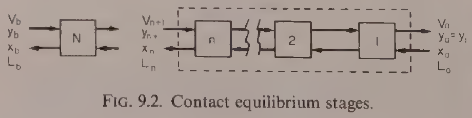
Diagram for Example 9.4: Earle's contact equilibrium stages. The single stage N at the left is the stage of this example: cream in at 8 ppm taint, steam in at 0.75 kg per kg of cream, cream out at 0.94 ppm. Reproduced from Earle, Fig. 9.2, p. 120.
Example 9.5: how many stages? Earle repeats the same deodorizing calculation as a multistage problem, stepping between the operating line and the equilibrium line on the McCabe-Thiele plot of Fig. 9.4. Starting from one terminal condition on the operating line, each step represents one contact stage, and the steps are drawn until the desired outlet concentration is reached. For the deodorizing duty of Example 9.4, the construction gives approximately three stages. That is the general lesson of the stage method: one stage does a lot when the equilibrium favours the transfer, and a few more stages, each repeating the same contact, carry the separation as far as it needs to go. The book's plot labels the equilibrium line yₙ = 7.5xₙ and the operating line yₙ₊₁ = 1.33xₙ - 0.43 in the coordinates of that figure; the step count of about three is the result the construction gives.
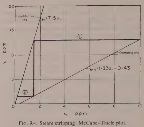
Diagram for Example 9.5: the McCabe-Thiele plot for steam stripping. The equilibrium line is yₙ = 7.5xₙ and the operating line is yₙ₊₁ = 1.33xₙ - 0.43; stepping between them gives approximately three stages. Reproduced from Earle, Fig. 9.4, p. 122.
Quick check
In Example 9.4, why does the taint fall eightfold in a single stage even though the steam flow is smaller than the cream flow?
Check your answer
Because the equilibrium ratio is 10 to 1 in favour of the steam: at equilibrium the steam holds ten times the taint concentration of the cream, so a modest steam flow can carry away most of the taint.
Try it yourself: one stage, then three
Take the numbers of Example 9.4 and change one thing at a time on paper: first double the steam flow to 1.5 kg per kg of cream, then halve the equilibrium ratio from 10 to 5. Work out the new outlet taint with the same equation, y₂ = x₁(L/V) + yₖ - xₖ(L/V), with y₁ = 10x₁. Which change helps more, more steam or a better equilibrium? That comparison is the designer's daily judgement: flow costs energy and solvent, while equilibrium is set by temperature, pressure and the choice of solvent.
5.6 Extraction and washing: the same idea in liquids and solids
Extraction is the same contact-equilibrium idea with different phases. A solvent is brought into contact with a solid or a liquid, the wanted component distributes itself between the phases according to equilibrium, and the enriched stream is taken away. Earle lists the food examples: edible oil extracted from seed, coffee extracted from beans with water, fatty acids extracted by liquid-liquid extraction, sucrose washed out of beet by water extraction. In the simple case of multistage oil extraction with a solvent, where equilibrium is reached in each stage, the concentration of oil is the same in the liquid leaving the stage as in the solid residue, so the equilibrium diagram is a straight line, y = x, and the stage calculation is straightforward.
The rate of extraction follows the same pattern as gas absorption. Earle gives dw/dθ = K_yA(y_s - y) (9.8), where y_s is the saturation concentration at the temperature of the system and y is the concentration in the bulk. Mixing helps because it keeps the local concentration equal to the mean bulk concentration, so there are no local pockets of high concentration to slow the transfer. Raising the temperature helps twice: it raises the coefficient K_y and it raises the solubility y_s. In extraction from a solid, part of the solute stays with the seed matrix, so the extraction can never be complete in one contact, and the plant is arranged in stages, often countercurrent, with the streams moving in opposite directions.
Washing is extraction where the wanted material is the solid left behind: the impurity is washed out, as in washing casein curd, where the curd starts at 60% water and is drained to 80% water between stages on an inclined screen, with lactose as the component being removed. The same stage arithmetic applies, with the wash water as the extracting stream.
Practical note: Earle is plain that stage-contact systems in which equilibrium has not been reached are beyond the scope of his book, and that in practice the shortfall is handled by assuming an efficiency for each stage. A real stage is never a perfect equilibrium stage, and the number of real stages is always larger than the number of theoretical stages. That efficiency, often well below 100%, is where pilot plant data earns its keep.
5.7 Crystallization: when a solution holds too much
Crystallization is used in the food industry for two purposes, and Brennan opens Chapter 8 by naming them. A liquid may be separated by crystallization into a solid and a liquid phase of different composition, one or both becoming products. Or no separation may be attempted and all the raw material stays in the product, as in a fondant or a fudge, where the size of the crystals decides the texture. In both cases the control of crystal size is the heart of the operation: uniform crystals separate cleanly from their mother liquor, and fine crystals give a smooth fondant while coarse ones give a gritty one. The texture of butter, too, depends on the size of the crystals formed during manufacture.
Solubility and the equilibrium diagram
Solubility is the maximum weight of anhydrous solute that will dissolve in 100 g of solvent, usually water in food work. It is a function of temperature, and for most food materials it rises as temperature rises. Pressure has very little effect on solubility. Earle's Fig. 9.1 shows the solubility of sodium nitrite in water rising from about 73 kg per 100 kg of water at 0°C to about 165 kg per 100 kg of water at 100°C, and the same rising shape holds for sucrose.
Brennan's equilibrium diagram for the sucrose-water system shows what cooling alone can and cannot do.
Figure 5.2: The equilibrium diagram for the sucrose-water system. Temperature in °C against concentration of sucrose in percent by weight in solution. The curve from the left meets the solubility curve at the eutectic point C, near 62% sucrose, and the dashed line θₕ marks the eutectic temperature. Below that line the equilibrium state is ice plus sucrose. (Brennan, Fig. 8.1, p. 151)
The diagram divides the field into four regions: Solution at the top, Solution + Ice on the left below the freezing curve, Solution + Sucrose on the right, and Ice + Sucrose below the dashed eutectic line. At a temperature just above the eutectic temperature θc the system is crystals of one component in equilibrium with a solution at the eutectic concentration C, near 62% sucrose, and just below θc the equilibrium state is a single solid phase of ice plus sucrose. The lesson Brennan draws is sharp: by cooling alone only a limited amount of ice or crystalline sucrose can be recovered pure, because the eutectic stops the separation. But only water is volatile in this system, so water can be driven off by heating, raising the sucrose concentration until crystallization occurs, and the solution could be evaporated to dryness with all the sucrose recovered crystalline, which cooling could never do.
Supersaturation: the metastable zone
A solution does not crystallize the moment it passes saturation. Cool it, or evaporate solvent from it, and it becomes supersaturated: it holds more solute than the saturation value at that temperature, yet no crystals appear. Brennan measures the degree of supersaturation by the coefficient S, the concentration of solute in the solvent divided by the concentration in a saturated solution at the same temperature. The solution is supersaturated when S is greater than 1.
Crystallization can be started by adding crystals of the solute, or crystals of similar structure, dust, gas bubbles, mechanical shock or ultrasonic vibration. Left alone, the rate at which nuclei form is very low at low supersaturation, then rises very steeply, then falls again at very high supersaturation, a fall the book attributes in part to rising viscosity. The rise is so steep that in practice a definite supersaturation S' can be named below which effectively no spontaneous nucleation occurs. That value defines the supersolubility curve.
Earle draws the same picture for sucrose in water, with the saturation curve below and the supersaturation curve above, and three regions between them.
Figure 5.3: Solubility and saturation curves for sucrose in water. Concentration in lb sucrose per lb water against temperature in °C. The lower solid curve is the solubility, or saturation, curve; the upper curve marked with crosses is the supersaturation curve. Between them lies the metastable region; below the solubility curve is the stable region. Curves traced from the printed figure; the axis values and labels are the book's. (Earle, Fig. 9.8, p. 131)
Below the saturation curve lies the stable region, where no crystal growth occurs. Between the saturation curve and the supersaturation curve lies the metastable region, where crystals will grow if seed crystals are added, but will not form on their own. Above the supersaturation curve, crystals form spontaneously and rapidly, without any outside help: this is spontaneous nucleation. Earle states the rule for growth plainly: the driving force that makes crystals grow is the concentration excess, the supersaturation, above the equilibrium saturation level, and the resistances are the resistance to mass transfer within the solution and the energy needed at the crystal surface for incoming molecules to orient themselves into the crystal lattice.
Brennan's supersolubility diagram for sucrose makes the same zones with the supersaturation coefficient made explicit.
Figure 5.4: Approximate supersolubility diagram for sucrose. Sucrose per 100 g water against temperature in °C. The dashed curve is the supersolubility curve and the solid curve is the solubility curve. Above the dashed curve is the labile zone, between the curves is the metastable zone, and below the solid curve is the undersaturated zone. Curves traced from the printed figure; the axis values, labels and zones are the book's. (Brennan, Fig. 8.3, p. 153)
The three zones have different rules. In the labile zone, above the supersolubility curve, nucleation happens spontaneously. In the metastable zone, between the curves, spontaneous nucleation is negligible, but seed crystals will grow. For the sucrose-water system the supersolubility curve sits near S = 1.3 and the boundary between the intermediate and metastable zones near S = 1.2, where S is the supersaturation coefficient. In the intermediate zone, just below the supersolubility curve, adding seed still makes nuclei appear in the solution, though spontaneous nucleation is still negligible. In impure sucrose solutions, as handled in sugar refining, the critical supersaturation that defines the supersolubility curve rises as the purity falls.
That gives the two industrial approaches to nucleation. One is to add finely divided seed crystals to a solution held in the metastable zone and grow them to finished size without any further nucleation. The mass of seed needed rises as the cube of the seed size, so very fine seed is needed to keep the seed mass reasonable. The other is to form nuclei from the solute already in the solution, either spontaneously in the labile zone or by shocking a solution in the intermediate zone with seed, and then either to hold the supersaturation high so nucleation continues, or to drop it into the metastable zone so nucleation stops and the existing nuclei grow. Which route is chosen depends on the relative rates of nucleation and crystal growth and on how tightly the finished crystal size must be controlled.
Example 9.8: how much salt crystallizes. Earle gives a short worked example that uses the solubility curve directly. A sodium chloride solution at 40°C has a concentration of 50% when the solubility of sodium chloride at this temperature is 36.6 g per 100 g water. Weight of salt in solution = 50 g per 100 g solution = 50 g per 50 g water, which is 100 g per 100 g water. Saturation concentration = 36.6 g per 100 g water. So the weight crystallized out = (100 - 36.6) g per 100 g water = 63.4 g per 100 g water, once crystallization has been started. To remove more salt the solution would have to be concentrated by removing water, or cooled to a lower temperature.
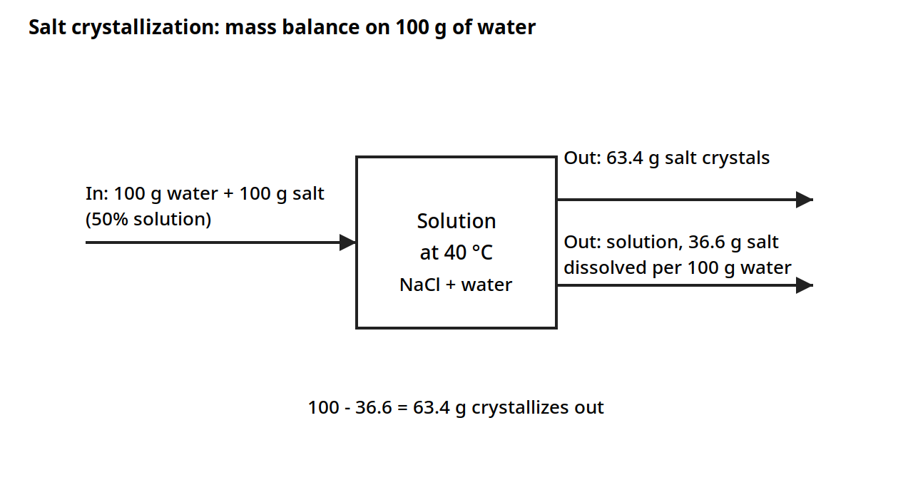
Diagram for Example 9.8: mass balance on a basis of 100 g of water. A 50% sodium chloride solution at 40 °C carries 100 g of salt per 100 g of water; the saturation concentration is 36.6 g per 100 g of water, so 63.4 g of salt crystallizes out. Drawn from the book's numbers; the book gives only this one sodium chloride point, so no solubility curve is drawn.
Crystal growth, polymorphism and food processes
Once nuclei exist, they grow by deposition of solute on their surfaces, and the growth rate depends on the supersaturation, on mass transfer to the surface, and on the surface itself. Crystals can also stick together into aggregates, trapping mother liquor in the gaps and lowering the purity of the solid. Stirring during crystallization reduces aggregation, as do surface active agents and a high dielectric constant in the solution. Aggregation is less of a problem in crystallizing sugar from impure syrups than from high purity syrups, because the impurities in the former are surface active and lower the surface tension.
Some substances crystallize in more than one form, with different molecular arrangements in the lattice and different physical properties. This is polymorphism, and it matters most in the food industry for fat crystallization. Many triglycerides can crystallize in several structures, each with a different melting point, and almost all triglyceride polymorphism is monotropic, meaning irreversible: a lower melting point crystal can only transform into a higher melting point form, never back. Fats supercool easily to the temperature of fusion of the lowest melting point form, crystallize rapidly in that least stable form, and then transform to the higher melting point forms at a rate that depends on temperature. Melt the fat and cool it again, and the low melting point crystals form again. Anyone who has watched chocolate bloom or a fat spread turn grainy has seen polymorphism doing its work.
Brennan describes the food processes that use crystallization with separation. Winterization of salad oils removes high melting point glycerides by slow fractional crystallization, so the oil does not turn cloudy in cold storage: cottonseed oil, for example, will crystallize at 40 to 45°F and turn turbid unless those glycerides are removed. The cooling is spread over two or three days, the degree of supercooling is kept low so nucleation stays slow, large crystals are grown because they entrain the least oil, and once nucleation has happened the oil is not stirred, so the crystals are not broken. Freeze concentration crystallizes ice out of liquid foods, which concentrates the liquid without any heat damage. It has been used for citrus juice concentrates, for concentrating alcoholic beverages and adjusting the alcohol content of wines, for vinegar, and as a preliminary concentration before freeze drying. Its limits are plain in the book: the degree of concentration achievable is limited by the eutectic, and the process is at present more expensive than evaporation. Ice crystals are separated by centrifugation, often in two or more stages, and may be washed with feed stock or melt water.
Where the solid is the wanted product, the prime examples are salt and sugar. The rate of crystal growth is far higher in salt solutions than in sugar solutions supercooled to the same extent, and salt solutions nucleate freely at very low supersaturations, while sugar solutions do not. So salt is crystallized in a continuous process with nucleation going on throughout, and crystals removed as they reach size, while sugar is crystallized by a batch method in which all nucleation is confined to the start. In coastal areas with high sunshine, sea water is evaporated in shallow salt pans by natural agencies; elsewhere factory methods evaporate brine at or just below its boiling point in open pans to give coarse salt.
Quick check
A sucrose solution sits between the solubility curve and the supersolubility curve. Will crystals appear on their own, and what happens if you add a few seed crystals?
Check your answer
No crystals appear on their own: that is the metastable zone, where spontaneous nucleation is negligible. Seed crystals will grow by deposition of solute on their surfaces until the solution concentration falls to the saturation line.
5.8 Adsorption and ion exchange: solids that catch solutes
Adsorption and ion exchange are mass transfer operations in which a solute in a fluid is transferred to a solid, either by being held on the solid's surface or by reacting with it. Ibarz treats them together in Chapter 22 because the mathematics of their columns is similar.
In adsorption the solute held is the adsorbate and the solid is the adsorbent. Adsorbents are porous solids with a large contact surface: activated carbon is widely used, and there are synthetic polymers called molecular sieves. The solute can be held by electric forces, by van der Waals forces, or by a chemical reaction. When the forces are van der Waals forces the adsorption is physical and usually reversible, and the solute can be held at any point of the surface. When it is a chemical reaction, chemisorption, the adsorbent has active points where the adsorbate is held. Adsorption is used to purify fluids that carry compounds giving unpleasant flavours or aromas. Ibarz gives two food examples: limonene, a compound that gives a bitter flavour to orange juice, can be removed by adsorption on polymers, and melanins and melanoidins, formed by enzymatic and nonenzymatic browning, can be removed by adsorption on activated carbon.
Ion exchange replaces ions in a solution with ions held in a solid called an exchange resin. It can be seen as a chemical adsorption, with exchange happening at defined points of the resin. Resins are anionic or cationic according to the ions they exchange. One of the most important applications is the desalination and conditioning of water.
Equilibrium: the isotherms
When adsorbent and fluid are left in contact, solute moves to the solid until a dynamic equilibrium is reached. At that point the fluid has a solute concentration C and the solid holds an amount m per unit mass. The function that gives m against C is the adsorption isotherm, and it can take several shapes: linear, favourable, irreversible, and others. Three equations describe the common shapes.
The Langmuir isotherm comes from a kinetic picture of one molecular layer: solute A in the fluid meets a free site S on the solid, and at equilibrium mₐ/m₀ = KCₐ/(1 + KCₐ) (22.3), where m₀ is the maximum amount the adsorbent can hold and K is the equilibrium constant. The Freundlich isotherm is an empirical equation, mₐ = K(Cₐ)ⁿ (22.4), with K and n found experimentally for each system and temperature. The BET isotherm, after Brunauer, Emmett and Teller, describes adsorption in several molecular layers, and for a gas it is written in terms of x = pₐ/pₐ°, the partial pressure over the vapour pressure of the pure solute, with B a constant for the interaction energy with the surface. When the number of layers is one, the BET equation reduces to the Langmuir form.
For ion exchange the equilibrium is written as a reaction, Aⁿ⁺ + R-B → Bⁿ⁺ + R-A, with an equilibrium constant K that the book calls the separation factor when it is expressed with the equivalent fractions of A in the liquid, Y = Cₐ/Cₐ₀, and in the resin, X = Eₐ/Eₘ: K = (1 - Y)X / (Y(1 - X)) (22.9). Here Eₐ is the equivalents of A per unit mass of dry resin and Eₘ is the maximum capacity of the resin.
Kinetics and operation
Three stages carry the solute to its resting place in adsorption: external transfer from the fluid to the surface, with flux N = k_F(C - Cᵢ) (22.10); diffusion inside the solid, with the flux set by the effective diffusivity Dₑ; and the adsorption step itself. Generally the first stage controls the process, so equilibrium can be assumed at the adsorption step. Ion exchange has five stages: external transfer of A to the resin surface, diffusion of A through the pores to the exchange points, the exchange reaction itself, diffusion of B back out through the pores, and external transfer of B to the solution. The slowest stage controls, and generally the diffusion stages or the external transfer stages control.
Operation can be in a single simple contact, repeated simple contacts, or countercurrent multiple contact, in batch or continuous form. The most common industrial form is the fixed-bed column, where the fluid flows through a bed of adsorbent or resin. As the bed loads, a zone of exchange moves down the column, and the book gives methods to calculate the height of that exchange zone, including the method of Rosen and the exchange zone method. The column is run until the solute first appears in the outlet, the breakthrough point, and then the bed is regenerated or replaced.
🤔 Pause and think: think of a jug of water passed through a carbon filter, or a water softener in a house. The water comes out tasting cleaner, but the filter does not last forever. What has the solid inside collected, where has it gone, and what tells you the bed is full? That is breakthrough, seen in a kitchen.
Quick check
What is the difference between physical adsorption and chemisorption, and which one is usually reversible?
Check your answer
Physical adsorption holds the solute by van der Waals forces at any point of the surface and is usually reversible. Chemisorption holds it by a chemical reaction at active points on the adsorbent.
5.9 Membrane separations: a barrier that chooses
A membrane separation puts a thin barrier between two streams and lets some components through while holding others back. Earle's Chapter 9 gives the food picture: reverse osmosis and ultrafiltration are the two main forms. In reverse osmosis, pressure is applied to overcome osmotic pressure and force water through the membrane, leaving dissolved solids behind. In ultrafiltration, larger molecules such as proteins are held back while water and small solutes pass. The driving force is a concentration or pressure difference across the membrane, and the rate is set by that driving force and by a mass transfer coefficient, in the same form as the other separations in this unit. The Sherwood number takes the place of the Nusselt number of heat transfer, and the Schmidt number takes the place of the Prandtl number, which is one more sign of the likeness between heat and mass transfer.
Membrane equipment is pumps, flow systems and membranes. Ultrafiltration membranes are set up in tubular form or in plates mounted like a filter press or a plate heat exchanger, with high flow rates over the surfaces and recirculation on the retentate side. Reverse osmosis needs mechanical strength for the high pressures, so flat disc membranes are stacked one above another, or very small diameter hollow filaments, around 0.04 mm, are used on plastic supports. A practical limit is bacterial growth: after a time the bacteria in the system, for example in the gel layer at the surface of an ultrafiltration membrane, grow so high that cleaning must be provided, and many membranes are not robust to mechanical disturbance or to extremes of pH that would give quicker and better cleaning.
Example 9.12: concentrating whey by ultrafiltration. Earle works a complete membrane design example. Whey from cheese manufacture is to have its protein concentration increased by a factor of 12 by ultrafiltration, to give an enriched fraction that can be dried to a 50% protein whey powder. The whey initially contains 6% of total solids, 12% of these being protein. Pilot scale measurements show a permeate flow of 30 kg m⁻² h⁻¹ can be expected. The plant must handle 30,000 kg in 6 hours. Assume the membrane rejection of the protein is over 99%.
Protein in the initial whey = 6 x 0.12 = 0.7%. Protein in the retentate = 12 x 0.7% = 8.6%. On a basis of 100 kg of whey, the mass balance is:
Table 5.3: Mass balance for ultrafiltration of whey, basis 100 kg (Earle Example 9.12)
| Stream | Water (kg) | Protein (kg) | Non-protein (kg) |
|---|---|---|---|
| Initial whey | 94 | 0.7 | 5.3 |
| Retentate | 6.7 | 0.7 | 0.7 |
| Permeate | 87.3 | 0.0 | 4.6 |
Water removed per 100 kg of whey = 87.3 kg. The plant must pass permeate at 30,000 x 87.3/(100 x 6) = 4,595 kg h⁻¹, and with a permeate rate of 30 kg m⁻² h⁻¹ the membrane area needed is 4,595/30 = 153 m². The non-protein rejection rate is 0.7/5.3 = 13%. So the membrane keeps nearly all the protein and lets most of the non-protein solids through with the water: a 153 m² membrane turns 30,000 kg of thin whey into a retentate at 8.6% protein, without any heat at all. That absence of heat is the point Earle closes on: membrane processes use only one apparent contact stage, they avoid the thermal damage that heat brings, and more extensive application can be expected as membranes, flow systems and pumps improve.
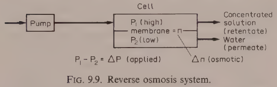
Diagram for Example 9.12: the reverse osmosis system, the same membrane arrangement as the ultrafiltration of this example: feed pumped into the cell, permeate through the membrane, concentrated retentate out. Reproduced from Earle, Fig. 9.9, p. 136.
Practical note: membrane separations are covered in full in Unit 10 of this subject, with Ibarz Chapter 10 as the main source. This section gives the contact-equilibrium view from Earle Chapter 9, so the reader can see membranes beside absorption, extraction and crystallization before the detailed design treatment.
5.10 What the books do and do not give
A careful reader should know the limits of the sources used for this unit. Ibarz Chapter 20 is a full design treatment of absorption, with equilibrium, films, packing, flooding, transfer units and plate columns, but it gives no worked examples inside the text, only problems at the end of the chapter. Earle Chapter 9 gives the worked examples used here, Examples 9.1 to 9.5, 9.8 and 9.12, but his text is a scanned book and its OCR is garbled in places: every number quoted from Earle in this unit was checked against the rendered page image before it was written down. Brennan Chapter 8 is a full treatment of crystallization, with the equilibrium and supersolubility diagrams, nucleation theory, polymorphism and food processes, but it has no worked numerical examples. Ibarz Chapter 22 gives the equilibrium, kinetics and stage operation of adsorption and ion exchange, with fixed-bed column methods, but no worked food example with numbers. The FPE papers listed in the outline for this unit, Moo-Young and Andre on mass transfer phenomena and Loncin on diffusion in solids, were not used as sources for the text above, because the unit is built from the three textbook chapters named in the outline.
Try it yourself: Look at three foods in a shop that were separated by the methods of this unit: a bag of sugar, a bottle of decaffeinated coffee or a fruit juice, and a tub of whey protein powder. Read the labels and ask, for each one: which component was moved, which phase did it move into, and what was the driving force? For the sugar, the answer is in the solubility curve. For the juice, it may be adsorption. For the powder, it may be a membrane. Write down your three answers in your own words. If a label does not say how the food was made, say so: a missing fact is a fact, not a gap to fill by guessing.
Key ideas to carry forward
- Mass transfer moves a component from high concentration to low, following Fick's law, and it stops when the phases reach equilibrium.
- Dalton's law, Raoult's law and Henry's law describe gas-liquid equilibrium; Henry's law, p = Hx, is the workhorse for dilute absorption, and warm liquid holds less gas than cold liquid.
- Mole fractions, not weight fractions, are the natural units for gas mixtures: 30% ethanol by weight is a mole fraction of 0.144, and air at 79 parts nitrogen to 21 parts oxygen has a mean molecular weight of 28.8, say 29.
- The double film theory puts a thin still film on each side of the interface, with equilibrium at the interface itself; the flux through each film is a coefficient times a driving force.
- Overall coefficients Kɢ and Kₗ replace the unmeasurable interface compositions, and the controlling resistance sits in the phase where the solute is least soluble: very soluble gases are gas-phase controlled, slightly soluble gases are liquid-phase controlled.
- In a packed absorption column the operating line has slope L'/G', the minimum solvent ratio is set where the operating line touches the equilibrium curve, and practice uses 25% above that minimum.
- Packing is chosen by specific surface, void fraction and packing factor; smaller packing gives more surface but a larger pressure drop, and the packing size must stay below one eighth of the column diameter.
- Flooding is the speed limit of a column: the loading velocity is about 0.6 times the flooding velocity, and gas velocities are usually about 1 m/s, from 0.3 to 5 m/s.
- Packing height is (height of a transfer unit) times (number of transfer units); Hɢ falls sharply with smaller rings while Hₗ stays near 0.5 to 0.7 m.
- Plate columns are used for large diameters, solids that would block packing, or very high liquid flows; their efficiency is 20 to 80%, and the Kremser equation gives the number of plates when the equilibrium line is straight.
- One stage of steam stripping cut a taint in cream from 8 ppm to 0.94 ppm, and about three stages complete the job in Earle's multistage example.
- Crystallization is governed by solubility and supersaturation: below the saturation curve nothing grows, in the metastable zone seed crystals grow but none form alone, and above the supersolubility curve nucleation is spontaneous. For sucrose the supersolubility curve sits near S = 1.3.
- Cooling alone cannot recover all the sucrose from a solution, because the eutectic stops it near 62% sucrose; evaporation to dryness can.
- Salt crystallizes continuously and sugar in batch, because salt nucleates freely at low supersaturation and grows fast, while sugar does not.
- Adsorption holds solutes on a porous solid by physical forces or by chemical reaction; the Langmuir, Freundlich and BET isotherms describe the equilibrium, and limonene in orange juice and browning compounds are food examples.
- Ion exchange swaps ions with a resin, and its equilibrium is described by the separation factor.
- Ultrafiltration raised whey protein from 0.7% to 8.6% with 153 m² of membrane for 30,000 kg in 6 hours, keeping over 99% of the protein and rejecting only 13% of the non-protein solids, with no heat.
Glossary
Mass transfer
The movement of a component from one place or phase to another, driven by a difference in concentration. Food tech example: carbon dioxide moving from a fizzy drink into the air when the bottle is opened.
Diffusion
The movement of molecules from high concentration to low concentration by their own motion, described by Fick's law. Food tech example: salt diffusing into a cucumber in brine.
Diffusivity
A number, D, that says how fast a component diffuses through a given material; large in gases, small in liquids. Food tech example: aroma compounds diffusing quickly through air above a cut apple and slowly through the apple flesh.
Equilibrium
The state in which the phases in contact have reached compositions that no longer change, so there is no net transfer. Food tech example: a gas above a liquid holding exactly the concentration that the liquid can support at that temperature and pressure.
Partial pressure
The pressure one component of a gas mixture would exert if it alone filled the whole volume. Food tech example: the partial pressure of carbon dioxide above a carbonated drink, which sets how much stays dissolved.
Henry's law
The rule that the partial pressure of a gas above a dilute solution is proportional to its mole fraction in the liquid, p = Hx. Food tech example: carbon dioxide in water at 25°C, with H = 1.6 x 10⁵ kPa per mole fraction.
Mole fraction
The fraction of the molecules in a mixture that belong to one component. Food tech example: a 30% by weight ethanol solution having an ethanol mole fraction of 0.144.
Double film theory
The model that mass transfer crosses a thin still film on each side of an interface by diffusion, with the two phases in equilibrium at the interface itself. Food tech example: a gas dissolving into a liquid film on packing in an absorption column.
Mass transfer coefficient
A number that links the flux across a film to the driving force across it, such as kₗ for the gas film and kₚ for the liquid film. Food tech example: the gas-phase coefficient kₗ = Dᵥ/RTL in absorption.
Overall mass transfer coefficient
A coefficient defined against the equilibrium compositions in the bulk phases, Kₗ or Kₚ, so that interface compositions, which cannot be measured, are not needed. Food tech example: the rate equation Nₚ = Kₚ(Cₜ - C) for absorption.
Absorption
A unit operation that separates one or more components from a gas mixture by dissolving them into a liquid. Food tech example: carbon dioxide removed from a gas mixture by passing it through water.
Desorption (stripping)
The reverse of absorption: a solute passes from the liquid into the gas phase. Food tech example: steam stripping a taint from cream, cutting it from 8 ppm to 0.94 ppm in one stage.
Operating line
The straight line on an equilibrium diagram that joins the compositions at the two ends of a column, with slope equal to the ratio of the two stream flows. Food tech example: the line of slope L'/G' on the Y-X diagram of an absorption column.
Packing
Inert solid pieces that fill an absorption column and give a large contact surface between gas and liquid. Food tech example: Raschig rings and Berl saddles in a packed tower.
Specific surface
The area a packing exposes to the fluid per unit volume of bed, in m²/m³. Food tech example: a 1/2 in. ceramic Raschig ring giving 416 m²/m³.
Void fraction (porosity)
The fraction of a packed bed volume not occupied by packing. Food tech example: 94% voids for a 3 in. ceramic Raschig ring bed.
Flooding
The condition in a column where the gas pressure holds the liquid up so it cannot flow down, and the pressure drop climbs steeply. Food tech example: the speed limit that sets the diameter of an absorption column.
Loading point
The gas velocity at which liquid begins to hold up in a packed bed, about 0.6 times the flooding velocity. Food tech example: the velocity a packed column is designed to run near, but not past.
Height of a transfer unit (HTU)
The height of packing that gives one transfer unit of separation, depending on flows and coefficients. Food tech example: Hₗ of 0.1 m for a 13 mm Raschig ring against 1.8 m for a 100 mm ring.
Number of transfer units (NTU)
A number that depends only on the inlet and outlet compositions and the equilibrium, saying how much separation is needed. Food tech example: packing height equals HTU times NTU.
Absorption factor
The ratio A = (L'/G')/H, which sets how easily a solute is absorbed; a large value gives high recovery. Food tech example: the factor used in the Kremser equation for plate columns.
Theoretical plate (stage)
An ideal contact stage in which the streams leaving are in equilibrium with each other. Food tech example: a plate in an absorption column counted by stepping between the operating line and the equilibrium curve.
Solubility
The maximum weight of a solute that will dissolve in 100 g of solvent at a given temperature. Food tech example: sodium chloride at 36.6 g per 100 g water at 40°C.
Supersaturation
A solution holding more solute than its saturation value at that temperature, measured by the coefficient S. Food tech example: a sucrose solution with S = 1.3, at the supersolubility curve.
Metastable zone
The range of concentrations between the solubility curve and the supersolubility curve, where seed crystals grow but no crystals form on their own. Food tech example: a sucrose solution held in the metastable zone while seed crystals grow to size.
Labile zone
The range above the supersolubility curve, where crystals form spontaneously. Food tech example: a sucrose solution taken into the labile zone so that nuclei appear without seed.
Nucleation
The formation of the first tiny crystals in a supersaturated solution. Food tech example: the start of sugar crystallization in a batch pan.
Seed crystal
A small crystal of the solute added to a supersaturated solution so that solute deposits on it and it grows. Food tech example: fine seed added to a fondant syrup held in the metastable zone.
Mother liquor
The liquid left behind after crystals have been separated from it. Food tech example: the syrup left after sugar crystals are centrifuged out.
Eutectic
The lowest temperature and the composition at which a mixture of two components freezes as one solid; for sucrose and water it sits near 62% sucrose. Food tech example: the point that limits how much sucrose cooling alone can recover.
Polymorphism
The ability of a substance to crystallize in more than one crystal form, with different melting points. Food tech example: triglycerides in fats crystallizing first in a low melting point form and then changing to higher melting point forms.
Winterization
Fractional crystallization by slow cooling to remove high melting point glycerides from an oil so it stays clear in cold storage. Food tech example: cottonseed oil winterized over two or three days.
Freeze concentration
Concentrating a liquid food by crystallizing ice out of it and removing the ice, with no heat. Food tech example: citrus juice concentrated by freezing and centrifugation.
Adsorption
The holding of a solute from a fluid on the surface of a porous solid. Food tech example: limonene removed from orange juice by adsorption on polymers.
Adsorbate
The solute held on an adsorbent. Food tech example: the bitter limonene held on a polymer adsorbent.
Adsorbent
The porous solid that holds the adsorbate, such as activated carbon. Food tech example: activated carbon removing browning compounds from a liquid.
Adsorption isotherm
The curve that gives the amount of solute held by an adsorbent against the concentration left in the fluid at equilibrium. Food tech example: the Langmuir isotherm, mₚ/m₀ = KCₚ/(1 + KCₚ).
Chemisorption
Adsorption by a chemical reaction at active points on the adsorbent, as opposed to physical adsorption by van der Waals forces. Food tech example: a solute bound chemically to active points on a solid.
Ion exchange
The replacement of ions in a solution by ions held in a solid resin. Food tech example: conditioning water by passing it through an exchange resin.
Separation factor
The equilibrium constant for ion exchange, K = (1 - Y)X/(Y(1 - X)), written with the equivalent fractions in the liquid and in the resin. Food tech example: the factor that describes how strongly a resin prefers one ion over another.
Breakthrough
The moment when a solute first appears in the outlet of a fixed-bed adsorption column, showing the bed is loaded. Food tech example: the point at which a carbon filter stops cleaning the water.
Reverse osmosis
A membrane process in which pressure forces water through a membrane, leaving dissolved solids behind. Food tech example: concentrating a liquid without heat by reverse osmosis.
Ultrafiltration
A membrane process that holds back large molecules such as proteins while water and small solutes pass. Food tech example: whey concentrated from 0.7% to 8.6% protein by ultrafiltration.
Retentate
The stream held back by a membrane, enriched in the components the membrane retains. Food tech example: the protein-rich stream from ultrafiltration of whey.
Permeate
The stream that passes through a membrane. Food tech example: the water and small solutes passing through an ultrafiltration membrane at 30 kg m⁻² h⁻¹.
References
- Ibarz, A., and Barbosa-Canovas, G. V., Unit Operations in Food Engineering, CRC Press, 2003. Chapter 4, Molecular Transport of Momentum, Energy, and Mass, Fick's law sections; Chapter 20, Absorption, including Figs. 20.1 to 20.12, Tables 20.1 and 20.2, Eqs. 20.1 to 20.79; Chapter 22, Adsorption and Ionic Exchange, including Fig. 22.1 and Eqs. 22.1 to 22.11.
- Earle, R. L., Unit Operations in Food Processing, 2nd edition, Pergamon Press, 1983. Chapter 9, Contact-Equilibrium Separation Processes, including Figs. 9.1 to 9.12, Examples 9.1 to 9.5, 9.8 and 9.12, Eqs. 9.1 to 9.20.
- Brennan, J. G., Butters, J. R., Cowell, N. D., and Lilly, A. E. V., Food Engineering Operations, Elsevier, 1969. Chapter 8, Crystallization, including Figs. 8.1 to 8.4, Eqs. 8.1 to 8.4.
- Whitman, W. G. (1923), double film theory, as cited in Ibarz and Barbosa-Canovas, Unit Operations in Food Engineering, Chapter 20.
- Barbosa-Canovas, G. V., and Vega-Mercado, H., Dehydration of Foods, Chapman and Hall, 1996, as cited in Ibarz and Barbosa-Canovas, Unit Operations in Food Engineering, Chapters 17 and 20.
- Costa, J., et al., Curso de Quimica Tecnica, Reverte, 1984, as cited in Ibarz and Barbosa-Canovas, Unit Operations in Food Engineering, Fig. 20.7.
- Coulson, J. M., and Richardson, J. F., Chemical Engineering, 1979, as cited in Ibarz and Barbosa-Canovas, Unit Operations in Food Engineering, Chapter 20, for the Semmelbauer correlations and the Morris and Jackson values.
- McCabe, W. L., and Thiele, E. W. (1925), graphical stage method, as cited in Earle, Unit Operations in Food Processing, Chapter 9.
- Perry, R. H., Chemical Engineers' Handbook, 1973, as cited in Earle, Unit Operations in Food Processing, Chapter 9, for vapour pressure data.
- Geankoplis, C. J., Transport Processes and Unit Operations, 1983, as cited in Ibarz and Barbosa-Canovas, Unit Operations in Food Engineering, Chapter 17.
Unit 6: Drying and Dehydration
Note
Unit 6: Drying and Dehydration
A bunch of grapes left in the sun turns into raisins. The grapes lose most of their water, shrink to a fraction of their weight, and keep for months without a fridge, while the fresh grapes would spoil in days. Nothing was added and nothing was cooked: water simply left, carried away by warm dry air. That is drying, the oldest preservation method there is, and it is also one of the most exacting pieces of engineering in a food factory, because the same hot air that removes water can scorch flavour, brown colour and harden the surface so the inside never dries at all. This unit follows the water out of the food, step by step.
Questions to think about
- Why does removing water preserve food, and how dry is dry enough?
- What is the difference between water a food holds loosely and water it holds tightly?
- Why does a wet surface dry at a steady rate, and then suddenly slow down?
- How do you read a psychrometric chart, and what does it tell you about the air in a dryer?
- How much heat does it take to dry a kilogram of food, and where does that heat go?
- Why does freeze dried coffee keep its aroma when hot air dried coffee does not?
6.1 Why dry food
Drying is one of the unit operations most commonly used for food preservation, and Ibarz notes that it has been used since prehistoric times because it gives foods longer lives. As populations grew, the demand for dried foods grew with them, and the drying industry grew in step, with military needs for light, long keeping rations driving many of the advances. The reasons are still the same today. Taking water out of a food slows microbes and slows the chemical reactions that spoil it. It also cuts weight and, in some cases, volume, which cuts the cost of packaging, handling, storage and transport. A sack of dried milk powder ships for a fraction of the cost of the same milk as liquid, and it needs no refrigeration on the way.
The books draw a line between two words that are often used as if they meant the same thing. Drying and dehydration are not synonyms. A food is considered dehydrated if it does not contain more than 2.5% water, while a dried food may contain more than 2.5% water. That 2.5% line matters because the last few percent of water are the hardest to remove and the most important for keeping quality: they are the water that microbes and browning reactions need.
Except for freeze drying, osmotic drying and vacuum drying, water is removed in most cases by blowing a flow of dry air over the food, which carries water from the surface of the product into the air stream. Drying does more than remove water, and the books are honest about the cost: it can destroy nutrients and set off enzymatic and nonenzymatic reactions, change colour and flavour, and harden texture. The engineering of drying is the art of removing the water fast enough to be economical, gently enough to keep the food worth eating, and evenly enough that no part is over dried while another part stays wet.
Quick check
What is the difference between a dried food and a dehydrated food in the book's definition?
Check your answer
A dehydrated food contains no more than 2.5% water. A dried food may contain more than 2.5% water.
6.2 The water inside a food: free, bound and in equilibrium
Not all the water in a food behaves the same way. Some of it is held loosely, almost as if it were free water in a dish, and it leaves easily. Some of it is held tightly by the food itself, and it leaves only with difficulty. The books describe the range of holding strengths rather than two neat boxes: water is held by forces that run from the very weak forces retaining surface moisture to very strong chemical bonds. The loosely held part can, for drying purposes, be treated as free water at the surface. The tightly held part is bound water, and as drying goes on the remaining water is bound more and more strongly, so the drying rate falls.
A hygroscopic material is one that contains bound water which exerts a vapour pressure lower than the vapour pressure of liquid water at the same temperature. Foods made mainly of carbohydrates behave this way, because the hydroxyl groups around the sugar molecules form hydrogen bonds with water molecules. In water soluble proteins, the polar amino acids sit on the outside of the molecule and the water hating groups sit inside, which lets the protein form hydrogen bonds with water and explains why such proteins dissolve. Fats and crystalline salts and sugars absorb almost no water when the relative humidity is low or moderate, while sugars in the amorphous form absorb more than in the crystalline form.
The key working idea is the equilibrium moisture content. Under a given vapour pressure of water in the surrounding air, a food settles at a moisture content in equilibrium with its surroundings, and it cannot be dried below that content by air at those conditions, however long it stays in the dryer. Earle's Fig. 7.4 plots equilibrium moisture against the relative humidity of the air for several foods, and the curves are S shaped. For potato at 20°C in air at 30% relative humidity, giving a water activity of 0.3, the equilibrium moisture content is 0.1 kg water per kg dry potato. It would not be possible to dry potatoes below 10% using an air dryer with air at 20°C and 30% relative humidity. Above about 80% relative humidity the equilibrium content of potato rises very rapidly. The curves differ between foods in shape and in amount, most strongly between 0 and 65% relative humidity, and the S shape is most pronounced, with the highest moisture at low humidities, for foods whose dry solids are high in protein, starch or other high molecular weight polymers.
Water moves inside the food by several mechanisms: capillary forces, diffusion of liquid down a concentration gradient, surface diffusion, diffusion of water vapour in pores filled with air, flow down a pressure gradient, and flow by vaporization and condensation of water. In the pores of rigid solids, capillary forces hold the water. In solids made of fine powder aggregates, osmotic pressure holds it. The drying rate at any moment depends on which of these mechanisms is slowest, and that changes as the food dries.
Practical note: the equilibrium moisture content is the floor of the whole operation. A dryer specification that asks for a final moisture below the equilibrium value for the drying air is not ambitious, it is impossible. The first check on any drying duty is to read the equilibrium moisture from the curve for the food at the temperature and humidity of the drying air.
6.3 The air side: psychrometry
Drying with hot air is a partnership between the food and the air, and the air must be understood first. Psychrometry is the study of air-water mixtures, and Ibarz Chapter 5 gives the working definitions, all referred to one kilogram of dry air.
Absolute humidity X is the mass of water per mass of dry air, in kg water per kg dry air. From the partial pressure of water vapour pᵥ and the total pressure P, X = 0.622 pᵥ/(P - pᵥ) (5.3), using the molecular weights of water, 18 kg/kmol, and air, 28.9 kg/kmol. When the air is saturated, pᵥ equals the saturation pressure pₛ, and X_saturation = 0.622 pₛ/(P - pₛ) (5.4).
Relative humidity φ is the ratio of the water vapour pressure in the air to the saturation pressure at the same temperature: φ = pᵥ/pₛ (5.5). Saturated air has φ = 1. The two humidities are linked by X = 0.622 φpₛ/(P - φpₛ) (5.6).
Percentage humidity is the ratio of the absolute humidity to the saturation humidity, X/X_saturation. Humid volume is the volume occupied by 1 kg of dry air plus the water vapour it contains, from the ideal gas law. Humid specific heat ŝ is the heat needed to raise 1 kg of dry air plus its water by 1°C: ŝ = ĉ_air + Xĉ_v (5.12), and with the mean values ĉ_air = 1 kJ/kg·°C and ĉ_v = 1.92 kJ/kg·°C, ŝ = 1 + 1.92X kJ per kg dry air per °C (5.13).
Humid enthalpy îɢ is the enthalpy of the dry air plus the enthalpy of its water vapour, referred to liquid water at 0°C and 1 atm. With λ₀ = 2,490 kJ/kg, the latent heat of vaporization of water at 0°C, îɢ = ŝT + λ₀X (5.16). The latent heat of vaporization itself falls as temperature rises, which is why the book gives the Regnault approximation λ = 2,538 - 2.91T kJ/kg, with T in °C.
Three temperatures describe the air, and they are easy to confuse, so the book defines each one. The dew temperature Tʀ is the temperature at which the air becomes saturated when it is cooled: the temperature at which condensation begins. The adiabatic saturation temperature Tₛ is the temperature at which air is saturated when it is cooled adiabatically. The humid temperature Tʜ, also called the wet bulb temperature, is the temperature reached by a small mass of water under adiabatic and steady conditions, exposed to an air stream of constant temperature, moisture and velocity. In the air-water system, for air velocities between 4 and 10 m/s, the humid temperature coincides with the saturation temperature. A wet bulb thermometer is a thermometer with its bulb wrapped in a wet wick and air blown past it: evaporation cools the bulb to the wet bulb temperature, and the difference between the dry bulb and the wet bulb, the wet bulb depression, tells the humidity.
The psychrometric chart puts all of this on one page. Ibarz presents the Mollier diagram in the form ŝT against X, with the product of humid specific heat and temperature on the vertical axis and absolute humidity on the horizontal axis. Isothermic lines are straight lines with slope 1.92T and intercept T, from ŝT = T + 1.92TX (5.17). The saturation curve φ = 1 bounds the chart: no point can sit beyond it, because air cannot hold more water than saturation at that temperature.
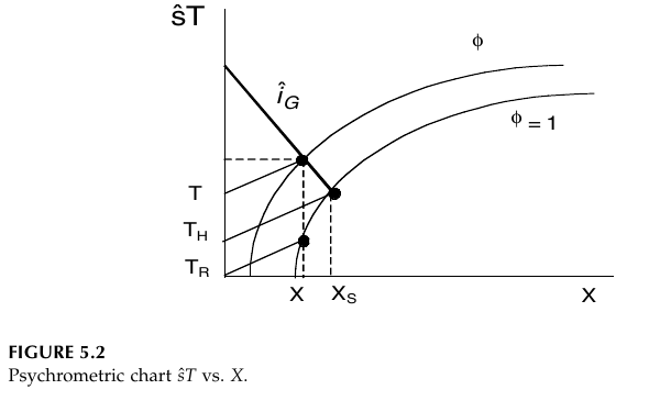
Figure 6.1: Psychrometric chart, ŝT against X. The product of humid specific heat and temperature is plotted against absolute humidity X. The curves are lines of constant relative humidity φ, with φ = 1 the saturation curve. The diagonal line is the isoenthalpic line îₗ. The points X and Xₛ mark the humidity and the saturation humidity, and T, Tₕ and Tₙ mark the dry bulb, humid (wet bulb) and dew temperatures. (Ibarz, Fig. 5.2, p. 70)
Heating air at constant humidity moves its point horizontally on the temperature-humidity chart: no water is added or removed, so the humidity stays the same while the temperature rises and the relative humidity falls. That is why heating is the first step in a dryer: hot air at low relative humidity has room to take up water. Cooling air at constant humidity moves the point horizontally the other way until it reaches the saturation curve at the dew point; further cooling follows the saturation line down, with water condensing out. Adiabatic saturation, the path air follows as it dries a wet solid with no outside heat, follows a line of constant wet bulb temperature: the air cools as it gives up heat to evaporate water, and its humidity rises by the same step.
Earle's worked examples in this section are all chart readings, and they show how much a chart can do. In Example 7.7, a wet bulb temperature of 20°C in air at a dry bulb temperature of 25°C, a wet bulb depression of 5°C, gives a relative humidity of about 64%, an enthalpy of 57 kJ kg⁻¹ and a specific volume of 0.862 m³ kg⁻¹. In Example 7.8, that same air heated to a dry bulb temperature of 40°C, at constant humidity, has an enthalpy of 73 kJ kg⁻¹, a specific volume of 0.906 m³ kg⁻¹ and a relative humidity of 27%. For a flow of 1,000 m³ h⁻¹, the mass is 1,000/0.906 = 1,104 kg, the enthalpy rise is 73 - 57 = 16 kJ kg⁻¹, and the heat needed is 1,104 x 16 kJ h⁻¹, which is 5 kW. Heating the air dropped its relative humidity from 64% to 27% without adding or removing a gram of water: that fall is the drying power the heater buys.
Quick check
Air at 25°C dry bulb and 20°C wet bulb is heated to 40°C with no water added or removed. What happens to its relative humidity, and why?
Check your answer
It falls, from about 64% to 27%. Heating at constant absolute humidity raises the saturation pressure, so the same amount of water vapour is a smaller fraction of what the air could hold.
Try it yourself: read the air in your kitchen
Take the temperature in a room with an ordinary thermometer, then wrap the bulb in a wet cloth, fan air past it with a piece of card, and read the lowest temperature it reaches. The difference between the two readings is the wet bulb depression. A big difference means dry air that would dry food quickly; a small difference means humid air that would dry food slowly. If you have a hygrometer, compare its reading with the relative humidity you estimate from the two temperatures. You have just used a psychrometer, the same instrument the books use to measure drying air.
6.4 The drying curve: steady, then slowing
Drying data are usually taken as the weight of the product against time, and from that curve the drying rate is found. The moisture content is defined on a dry basis: Y_t = (w_T - w_S)/w_S (17.9), where w_T is the total weight at a given time and w_S is the weight of dry solids. The free moisture content is Y = Y_t - Y_eq (17.10), the moisture above the equilibrium value. The drying rate R is proportional to the change of moisture with time, R ∝ dY/dt, and in full R = -(w'_S/A)(dY/dt) (17.12), where w'_S is the flow of dry solids and A is the drying surface area.
Plotted against free moisture, the drying rate gives the curve that governs the whole subject.
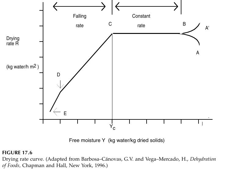
Figure 6.2: Drying rate curve. Drying rate R in kg water per h per m² against free moisture Y in kg water per kg dried solids. Points A and A' are the starting points for a cold and a hot material, B is the point where the surface reaches its equilibrium temperature, B to C is the constant rate period, C is the critical moisture Yₕ where the falling rate period begins, D is the point where the surface is completely dry, and E is the end of drying. (Ibarz, Fig. 17.6, p. 579)
The curve reads from right to left, because moisture falls as drying goes on. Points A and A' are the starting points for a cold and a hot material. Point B is where the surface reaches its equilibrium temperature, and the short time from A or A' to B is usually small and commonly neglected in drying time calculations. From B to C the rate is constant: this is the constant rate period, when unbound water is being removed. The surface stays wet, the water activity at the surface stays close to one, and water moves from the interior fast enough to replace what evaporates. In porous solids the water removed from the surface is made up by flow from inside. The surface temperature sits close to the wet bulb temperature, and the water behaves as if the solid were not there.
At point C the rate can no longer be held constant, and the falling rate period begins. The critical moisture content Yc is the moisture at C. The water activity at the surface falls below one, and the rate is now governed by the movement of water and water vapour inside the solid. The first stage of the falling rate period runs from C to D, while wet patches on the surface shrink until the surface is completely dry at D. The second stage runs from D to E, with the surface dry and the evaporation plane moving into the interior of the solid. Heat must travel through the solid to the evaporation plane, and the vapour produced must travel back out through the solid to the surface. Sometimes the two falling rate stages are not clearly distinct. The amount of water removed in the falling rate period may be small, but the time it takes may be long, because the rate is low.
Brennan draws the same story in three plots together, and the three views make the shape easier to remember.
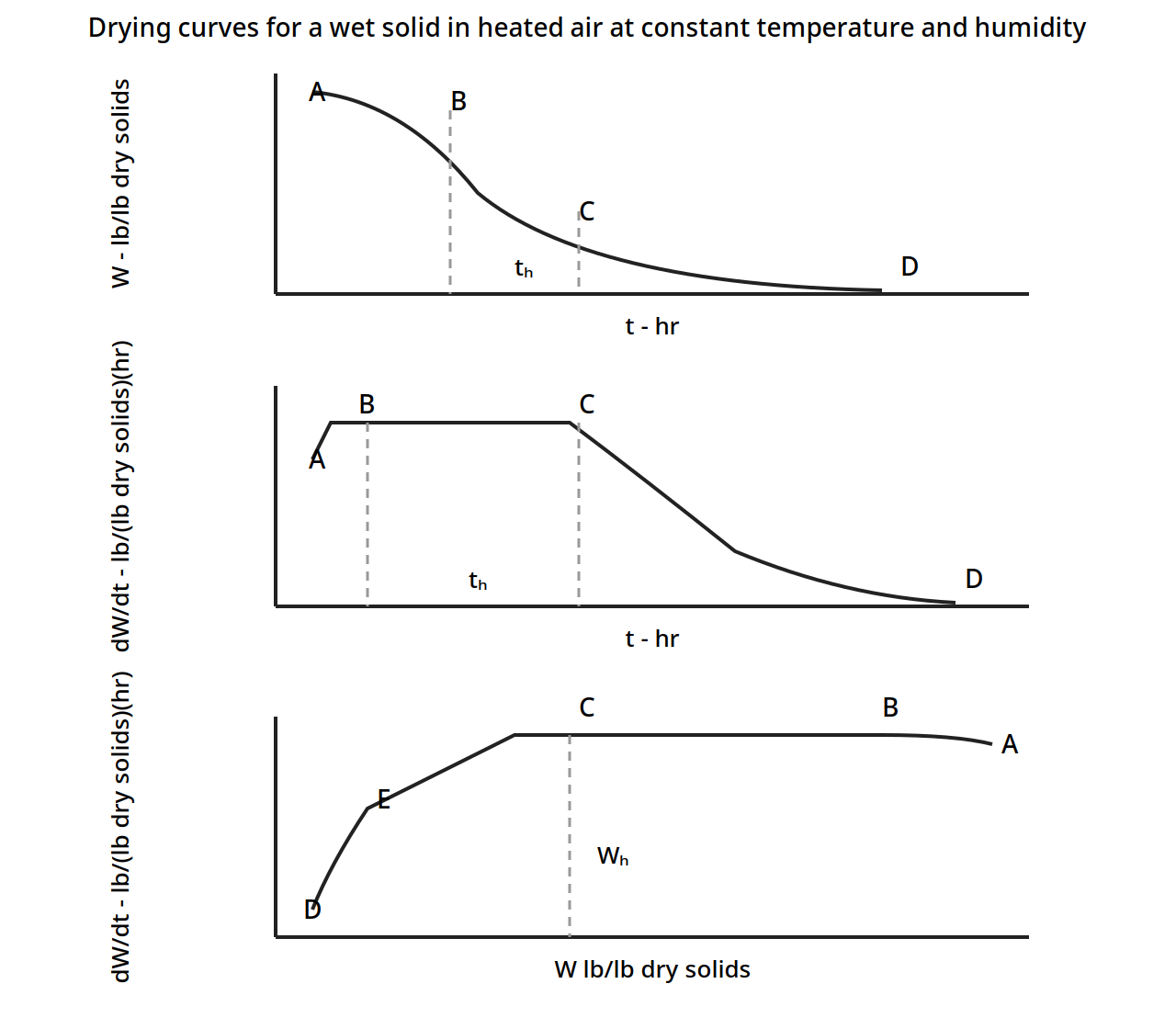
Figure 6.3: Drying curves for a wet solid in heated air at constant temperature and humidity. Top: moisture W against time t. Middle: drying rate dW/dt against time t, showing the constant rate plateau from B to C. Bottom: drying rate dW/dt against moisture W, showing the constant rate plateau from C to B and the critical moisture Wₕ. The critical time tₕ is marked on the first two plots. (Brennan, Fig. 12.2, p. 247)
Earle adds two facts that every food dryer must respect. First, the change from constant rate to falling rate happens at different moisture contents for different foods, but for many foods it happens when the moisture is in equilibrium with air of 58 to 65% relative humidity, that is at a water activity a_w of 0.58 to 0.65. That moisture is the critical moisture content Xc. Second, many foods, such as potato, do not show a true constant rate period at all: they show a slowly and steadily declining rate with a sharp break, and the constant rate idea is still a useful approximation.
The generalized drying curve makes the same point without any particular food in mind. Earle's Fig. 7.7 plots the relative drying rate, the rate divided by the constant rate, against the relative moisture content, X/Xc.
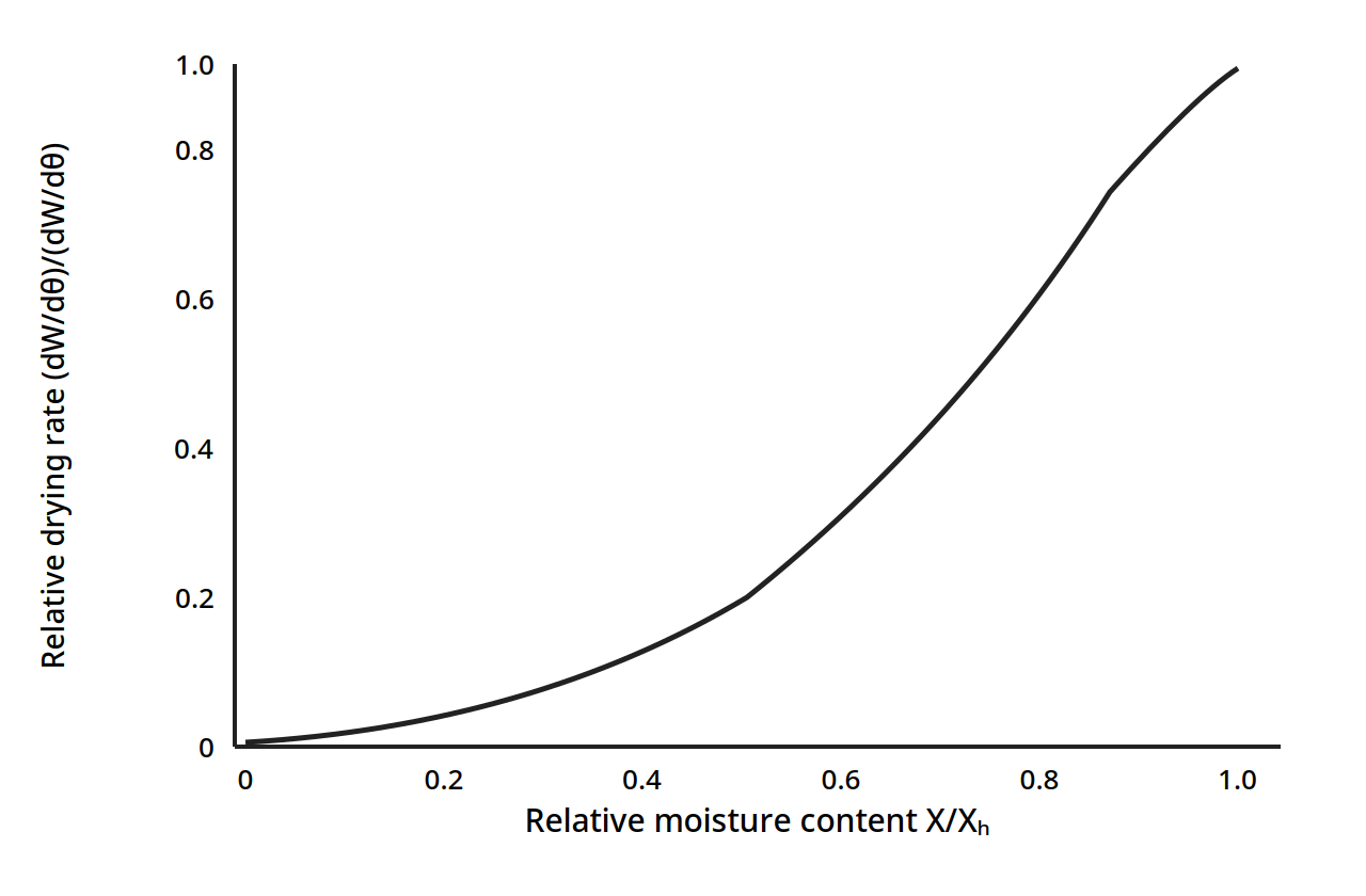
Figure 6.4: Generalized drying curve. Relative drying rate against relative moisture content X/Xₕ. At the critical moisture, X/Xₕ = 1.0, the relative rate is 1.0; below the critical moisture the rate falls away, at first slowly and then steeply. (Earle, Fig. 7.7, p. 96)
At the critical moisture the relative rate is 1.0, and below it the rate falls away in a curve that is the same shape for many foods once it is scaled this way. That is why the critical moisture is worth finding for each food: it divides the drying into the part the air controls and the part the food controls.
The constant rate period, in equations
During the constant rate period the surface stays saturated with water, and only two transfers matter: heat from the hot air to the surface, and mass from the surface to the hot air. With convection only, q = hA(T - T_w) (17.13), where h is the heat transfer coefficient, A the area, T the air temperature and T_w the wet bulb temperature. The mass flux is Nₐ = k_y(X_w - X) (17.14), where X_w is the humidity of air at the surface and X is the humidity of the air stream. The heat that evaporates the water is q = NₐMₐλ_wA (17.15), with Mₐ the molecular weight of water and λ_w the latent heat of vaporization at T_w. Putting them together gives the constant drying rate two ways:
R_c = k_yM_b(X_w - X) (17.16) and R_c = h(T - T_w)/λ_w (17.17)
where M_b is the molecular weight of air. The two must agree, because the heat arriving and the water leaving are the same event seen from two sides. If there is no conduction or radiation, the temperature of the solid during the constant rate period is the wet bulb temperature. Brennan gives the same result in the form [dw/dt]_c = -K_gA(p_s - p_a) (12.1), where p_s is the vapour pressure at the surface and p_a is the vapour pressure in the air: the driving force is the vapour pressure difference between the drying surface and the main stream of the drying air.
The falling rate period, and diffusion
Once the moisture falls below the critical value, the rate is set by the movement of water inside the solid, and Fick's law returns in its time dependent form:
∂Y/∂t = D_eff ∂²Y/∂x² (17.23)
where Y is the moisture content, t is time, x is the distance in the direction of transfer, and D_eff is the effective diffusion coefficient. The book gives the solutions for a slab, a cylinder and a sphere. For a slab the moisture ratio is a sum of exponentials in D_eff t/L², where L is the thickness; for a sphere it is a sum in D_eff t/r², where r is the radius. The effective diffusivity is found experimentally from drying data: plotting ln Γ against time, where Γ is the moisture ratio (Y - Y_s)/(Y₀ - Y_s), the slope of the straight section gives D_eff. Table 6.1 gives the book's values, which span three orders of magnitude: water moves far more easily through some foods than others, and that is why drying times differ so much between foods.
Table 6.1: Effective diffusivity of some food products (Ibarz Table 17.1)
| Food | Temperature (°C) | Effective diffusivity D_eff (m²/s) |
|---|---|---|
| Whole milk, foam | 50 | 2.0 x 10⁻⁹ |
| Whole milk, foam | 40 | 1.4 x 10⁻⁹ |
| Whole milk, foam | 35 | 8.5 x 10⁻¹⁰ |
| Apples | 66 | 6.40 x 10⁻⁹ |
| Freeze-dried apples | 25 | 2.43 x 10⁻¹⁰ |
| Raisins | 25 | 4.17 x 10⁻¹¹ |
| Potatoes | 54 | 2.58 x 10⁻¹¹ |
| Potatoes | 60 | 3.94 x 10⁻¹¹ |
| Potatoes | 65.5 | 4.37 x 10⁻¹¹ |
| Potatoes | 68.8 | 6.36 x 10⁻¹¹ |
| Pears (slabs) | 66 | 9.63 x 10⁻¹⁰ |
| Veal, freeze-dried powder | 25 | 3.07 x 10⁻¹¹ |
| Carrot cubes | 40 | 6.75 x 10⁻¹¹ |
| Carrot cubes | 60 | 12.1 x 10⁻¹¹ |
| Carrot cubes | 80 | 17.9 x 10⁻¹¹ |
| Carrot cubes | 100 | 24.1 x 10⁻¹¹ |
Table 6.1: Effective diffusivity of some food products. Source: Okos et al., in Heldman and Lund, Handbook of Food Engineering, 1992, as cited in Ibarz, Table 17.1, p. 585.
Two patterns stand out. Diffusivity rises with temperature: carrot cubes go from 6.75 x 10⁻¹¹ m²/s at 40°C to 24.1 x 10⁻¹¹ m²/s at 100°C, nearly four times faster. And it varies hugely between foods: apples at 66°C, 6.40 x 10⁻⁹ m²/s, let water move about 250 times faster than potatoes at 54°C, 2.58 x 10⁻¹¹ m²/s. A dryer sized for apples will not dry potatoes in anything like the same time.
Quick check
Why does the drying rate fall in the falling rate period, even though the air is just as hot and dry as before?
Check your answer
Because the surface is no longer wet: the rate is now set by how fast water can move through the inside of the solid to the surface, by diffusion, and that internal movement is slow.
6.5 How much heat does drying take
Most of the heat in drying goes to evaporating water, and the latent heat of vaporization is the biggest number in the whole calculation. Earle's Table 7.1 gives it at pressures from 1 kPa up to 500 kPa, and the pattern is simple: the lower the pressure, the higher the latent heat and the lower the boiling temperature.
Table 6.2: Latent heat of water at various pressures and saturation temperatures (Earle Table 7.1)
| Pressure (kPa) | Saturation temperature (°C) | Latent heat (kJ/kg) |
|---|---|---|
| 1 | 7 | 2485 |
| 2 | 18 | 2460 |
| 5 | 33 | 2424 |
| 10 | 46 | 2393 |
| 20 | 60 | 2358 |
| 50 | 81 | 2305 |
| 100 | 99.6 | 2258 |
| 101.35 (1 atm) | 100 | 2257 |
| 110 | 102 | 2244 |
| 120 | 105 | 2238 |
| 200 | 120 | 2202 |
| 500 | 152 | 2109 |
Worked example 6.1: drying a food at atmospheric pressure (Earle Example 7.1)
A food with 80% water is dried to 10% moisture. The initial temperature is 21°C, the latent heat at 100°C is 2,257 kJ kg⁻¹, the specific heat of the food is 3.8 kJ kg⁻¹ °C⁻¹ and of water is 4.186 kJ kg⁻¹ °C⁻¹.
Per kg of raw material, the solids are 0.20 kg. At 10% moisture the final mass is 0.20/0.90 = 0.222 kg, so the water lost is 1 - 0.222 = 0.778 kg per kg of raw material. The heat needed is the sensible heat to warm the food to 100°C plus the latent heat to evaporate the water:
Heat = (100 - 21) x 3.8 + 0.778 x 2,257 = 300.2 + 1,755.9 = 2,056 kJ per kg of raw material.
Per kg of water removed, that is 2,056/0.778 = 2,643 kJ kg⁻¹. The sensible heat is only about 15% of the total: evaporation dominates, as it always does in drying.
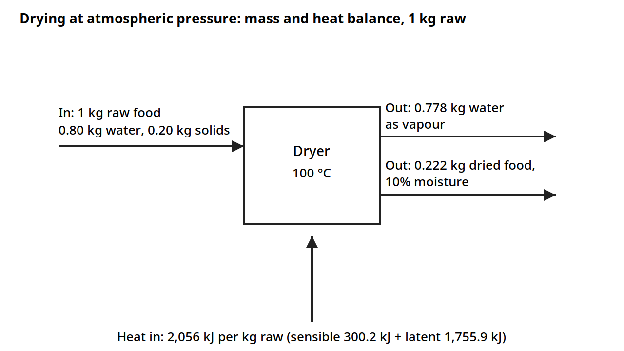
Diagram for Worked example 6.1 (Earle Example 7.1): mass and heat balance on 1 kg of raw food. The food is 80% water; drying to 10% moisture removes 0.778 kg of water, leaving 0.222 kg of dried food. Heat: 2,056 kJ per kg of raw food, 2,643 kJ per kg of water removed. Drawn from the book's numbers.
Worked example 6.2: vacuum drying (Earle Example 7.2)
The same food dried at 60°C in a vacuum of 81.4 kPa, giving an absolute pressure of 20 kPa. At 60°C the latent heat is 2,358 kJ kg⁻¹ from Table 6.2.
Heat = (60 - 21) x 3.8 + 0.778 x 2,358 = 148.2 + 1,834.5 = 1,983 kJ per kg of raw material.
The total is slightly less than at atmospheric pressure, and the food never gets hotter than 60°C, which is kinder to flavour and nutrients. The trade is the cost of the vacuum equipment and the larger latent heat at low pressure, which partly offsets the saving in sensible heat.
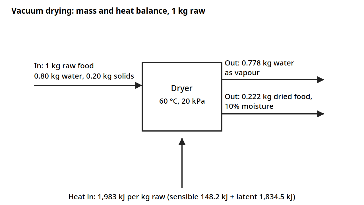
Diagram for Worked example 6.2 (Earle Example 7.2): the same balance at 60 °C under vacuum (81.4 kPa vacuum, 20 kPa absolute). The latent heat at 60 °C is 2,358 kJ kg⁻¹, and the heat needed is 1,983 kJ per kg of raw food. Drawn from the book's numbers.
Worked example 6.3: freeze drying (Earle Example 7.3)
The same food freeze dried at 0°C. The latent heat of sublimation of ice is 2,838 kJ kg⁻¹, higher than the latent heat of evaporation.
Heat = 0.778 x 2,838 = 2,208 kJ per kg of raw material.
Freeze drying takes more heat per kg of raw material than either of the other two, and it also needs refrigeration and vacuum, so it is the most expensive way to dry. It earns its place because the product never melts, never collapses, and keeps its shape, colour and aroma: the water leaves as vapour from the solid ice, so the structure stays open and porous.
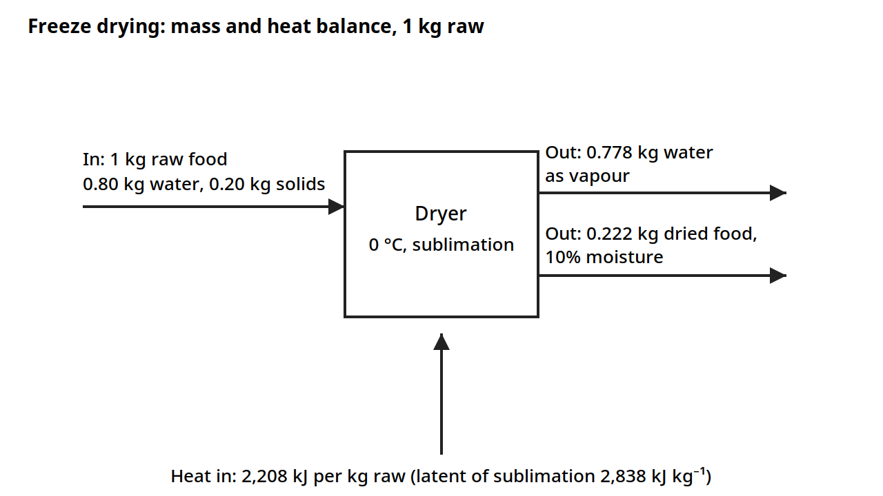
Diagram for Worked example 6.3 (Earle Example 7.3): the same balance for freeze drying at 0 °C. The water leaves as vapour from solid ice, so the heat is the latent heat of sublimation alone, 2,208 kJ per kg of raw food. Drawn from the book's numbers.
Quick check
A food is dried from 80% water to 10% moisture. Why is the heat needed per kg of water removed, 2,643 kJ/kg, higher than the latent heat of vaporization alone, 2,257 kJ/kg?
Check your answer
Because the food must first be warmed from 21°C to the drying temperature, and that sensible heat adds to the latent heat of evaporation.
6.6 How long will it take
Drying time is found in two parts: the constant rate time and the falling rate time, added together.
The constant rate time, from moisture Y₁ to the critical moisture Yc, is t_c = (w_S/R_cA)(Y₁ - Yc) (17.32), where w_S is the dry solids, R_c the constant drying rate, and A the area. It is simply the water to be removed divided by the rate at which water leaves.
The falling rate time depends on which model describes the food. For a slab of half thickness L, the first falling rate stage time is t_D = -(L²/D_eff)(π²/4) ln[(Y₂ - Y_s)/(Y₁ - Y_s)] in the form of Eq. 17.35, and for the second falling rate stage, where the evaporation plane has moved inside, t_D = (L²/D_eff) ln[(Y₁ - Y_s)/(Y₂ - Y_s)] in the form of Eq. 17.36, where Y_s is the surface moisture. The total drying time is t_S = t_C + t_D.
For a bed dryer, where air flows through a bed of solids, the books give the heat and mass balances that set the drying time and the air requirement: the water removed equals the change in the air's humidity times the air flow, and the heat supplied equals the change in the air's enthalpy times the air flow, with the heat used to evaporate water and to warm the solids. For a continuous countercurrent dryer the same balances apply stage by stage, with the solids entering wet and leaving dry while the air enters dry and leaves wet, and the books give the equations for the moisture and temperature profiles along the dryer (Eqs. 17.52 to 17.56). In all of these, the same two quantities govern the answer: how much water must leave, and how much heat the air can carry to the food and carry away as vapour.
Practical note: the constant rate period is usually the fast part and the falling rate period the slow part. A dryer sized only on the constant rate will be too small. Always size on the total time, and remember that the falling rate time grows with the square of the thickness: halving the slice thickness cuts the diffusion time to a quarter.
6.7 The dryers
A dryer has three parts: a feeder that presents the food to the drying air, a heater that warms the air, and a collector that catches the dried product and, where needed, the dust. The heater may heat the air directly, with the hot combustion gases mixing with the air, at temperatures up to 648 to 760°C, or indirectly, with a heat exchanger, at temperatures up to 425°C. The collector may be a cyclone, a bag filter or a wet washer. The choice of dryer depends on the form of the food: liquid, paste, pieces, or powder, and on how delicate it is.
Chamber and bed dryers
In a chamber dryer, the food sits on trays in a chamber and hot air is blown over it. In a bed dryer, air flows through a bed of pieces. Both are batch or semi continuous, and both are used for pieces of fruit, vegetables and meat, and for foods that cannot be pumped. The books give the balances for a bed dryer in Eqs. 17.43 to 17.48, linking the air flow, the humidity rise, the heat supplied and the water removed.
Spray drying
Spray drying turns a liquid into a powder in seconds. The liquid is atomized into fine droplets, sprayed into a stream of hot air, and the droplets dry as they fall, before they can hit a wall and stick. It was first used around 1900 for dry milk, and later for eggs and coffee. The droplet size sets the drying time and the powder size, and it is controlled by the atomizer. For a pressure nozzle, the droplet size falls as the pressure rises and as the feed rate falls, and it rises with the viscosity and surface tension of the feed (Table 17.2). For a rotary atomizer, a spinning disk throws the liquid off its edge, and the droplet size depends on the disk speed, the feed rate, the viscosity, the surface tension and the density, with the disk speed the strongest influence, an exponent of 0.55 to 0.80 (Table 17.3).
Table 6.3: Droplet size against process variables for a pressure nozzle (Ibarz Table 17.2)
| Variable | Effect on droplet size |
|---|---|
| Pressure | Droplet size decreases as pressure increases |
| Feed rate | Droplet size increases as feed rate increases |
| Viscosity | Droplet size increases as viscosity increases |
| Surface tension | Droplet size increases as surface tension increases |
The rotary atomizer is sized by Eq. 17.73, with constants that depend on the disk speed and the blade load, in kg per h per m of disk edge. Table 6.4 gives them.
Table 6.4: Constants for Eq. 17.73, rotary atomizer (Ibarz Table 17.4)
| Disk speed (m/s) | Blade load (kg/h·m) | a | b | d | K x 10⁴ |
|---|---|---|---|---|---|
| 85-115 | 250 | 0.24 | 0.82 | 0.24 | 1.4 |
| 85-180 | 250-1500 | 0.2 | 0.8 | 0.2 | 1.6 |
| 180-300 | 1000-3000 | 0.12 | 0.77 | 0.12 | 1.25 |
| 85-140 | 3000-60000 | 0.12 | 0.8 | 0.12 | 1.2 |
Table 6.4: Constants for the rotary atomizer droplet size equation. Source: Masters, Spray Drying Handbook, 1991, as cited in Ibarz, Table 17.4, p. 590.
Pneumatic atomizers use a high velocity air stream to break the liquid into droplets. The book notes that the ratio of air to liquid mass flow, w_air/w_liq, below 0.1 gives deteriorating atomization, and 10 is the upper limit (Table 17.5).
Freeze drying
Freeze drying has two stages. First the food is frozen. Then the pressure is dropped below the triple point of water, 627 Pa at 0°C, and heat is supplied so the ice sublimes directly to vapour, without melting. Because the water never becomes liquid, the structure does not collapse: the dried product keeps its shape, and the pores left by the ice make it rehydrate fast. The product is typically 10 to 15% of its original weight, with moisture below 2%, and it needs no refrigeration in storage. The process was developed in the 1940s for drying plasma and blood, and it is now used for coffee, fruits, vegetables and meats where quality justifies the cost.
During the second stage, secondary drying, the product must be kept below 30 to 50°C to prevent collapse of the dried structure. The rate depends on the thermal conductivity of the dried layer and on the sublimation temperature of the product, both given in Table 6.5.
Table 6.5: Thermal conductivity and sublimation temperature for freeze drying (Ibarz Table 17.6)
| Product | Thermal conductivity k (W/m·K) | Sublimation temperature T_sub (°C) |
|---|---|---|
| Coffee extract 25% | 0.033 | -23 |
| Gelatin | 0.016 | - |
| Milk | 0.022 | - |
| Apple | 0.016-0.035 | -7 |
| Peach | 0.016 | - |
| Turkey | 0.014 | - |
| Mushrooms | 0.010 | - |
| Veal | 0.035-0.038 | -14 |
| Shrimp | - | -18 |
| Whole egg | - | -17 |
| Chicken | - | -21 |
| Salmon | - | -29 |
| Carrot | - | -25 |
Table 6.5: Thermal conductivity of the dried layer and sublimation temperature for some foods. Source: Schwartzberg, 1982, as cited in Ibarz, Table 17.6, p. 595. A dash means the book gives no value for that cell.
The thermal conductivities are tiny, around 0.01 to 0.04 W/m·K, which is why freeze drying is slow: heat creeps through the dried layer to the ice front. The sublimation temperatures are all well below zero, from -7°C for apple to -29°C for salmon, which is why the product stays cold and its aroma stays put.
Other drying methods
The book closes the chapter with other types of drying, each suited to a particular food or situation: osmotic dehydration, where water is drawn out by a concentrated sugar or salt solution before air drying; solar drying, where the sun supplies the heat; drum drying, where a thin film of liquid dries on a hot rotating drum; microwave drying, where the heat is generated inside the food itself; and fluidized bed drying, where the pieces are suspended in a stream of hot air so that every surface sees the air. The chapter gives each of these briefly, and the choice between them turns on the same questions as always: the form of the food, the moisture to be removed, the quality to be kept, and the cost that can be borne.
6.8 Worked examples: sizing the air and the heat
The chart examples in section 6.3 show how to read the air. These examples show how to use those readings to size a dryer.
Worked example 6.4: how much air to remove a given amount of water (Earle Example 7.9)
Air at 60°C and 8% relative humidity enters a dryer and leaves at 35°C. From the chart, the inlet humidity is 0.010 kg kg⁻¹ and the specific volume is 0.96 m³ kg⁻¹. The outlet humidity is 0.0207 kg kg⁻¹. The water removed is 0.0207 - 0.010 = 0.0107 kg per kg of air. To remove 20 kg of water per hour, the air needed is 20/0.0107 = 1,869 kg h⁻¹, which at 0.96 m³ kg⁻¹ is 1,794 m³ h⁻¹. The answer is set by the difference between the outlet and inlet humidities: the wider that gap, the less air is needed.
The psychrometric chart (Figure 6.1) with the readings of this example: inlet air at 60 °C and 8% relative humidity, 0.010 kg kg⁻¹; outlet air at 35 °C, 0.0207 kg kg⁻¹. The water removed, 0.0107 kg per kg of air, is the gap between the two humidities.
Worked example 6.5: finding the relative humidity from the dew point (Earle Example 7.10)
Air leaves a dryer at 45°C with a dew point of 40°C. From the chart, the relative humidity is 76%. The dew point is a direct measure of how much water the air holds: air at 45°C that starts condensing at 40°C is nearly saturated.
The psychrometric chart (Figure 6.1) with the reading of this example: air leaving the dryer at 45 °C with a dew point of 40 °C, 76% relative humidity.
Worked example 6.6: a two stage tray dryer (Earle Example 7.11)
Air at 1,800 m³ h⁻¹, 18°C and 50% relative humidity is heated to 140°C, passed over trays, leaves at 60% relative humidity, is reheated to 140°C and passed over a second set of trays, leaving again at 60% relative humidity. From the chart, the initial humidity is 0.0062 kg kg⁻¹, the specific volume is 0.834 m³ kg⁻¹ and the enthalpy is 35 kJ kg⁻¹. Heated to 140°C the enthalpy is 160 kJ kg⁻¹. Following the wet bulb line to 60% relative humidity, the air leaves the first trays at 48°C with a humidity of 0.045 kg kg⁻¹. Reheated to 140°C, the enthalpy is 268 kJ kg⁻¹. Following the wet bulb line to 60% relative humidity again, the humidity is 0.082 kg kg⁻¹.
The total energy used is ΔH = 268 - 35 = 233 kJ kg⁻¹. The total water removed is ΔY = 0.082 - 0.0064 = 0.0756 kg kg⁻¹. The mass flow of air is 1,800/0.834 = 2,158 kg h⁻¹, which is 0.6 kg s⁻¹. The energy is 233 x 0.6 = 140 kW, and the water removed is 0.6 x 0.0756 = 0.045 kg s⁻¹, which is 163 kg h⁻¹. The exit air temperature is 60°C.
A printed inconsistency to note: the book states the initial humidity as 0.0062 kg kg⁻¹ but computes the water removed with 0.0064 kg kg⁻¹, giving ΔY = 0.0756 kg kg⁻¹. Using 0.0062, the difference would be 0.0758 kg kg⁻¹ and the water removed 163.7 kg h⁻¹. The difference is small, about 0.4%, and the book's own computed figures are given above as printed.
The psychrometric chart (Figure 6.1) with the readings of this example: inlet air at 18 °C and 50% relative humidity, 0.0062 kg kg⁻¹, heated to 140 °C and passed over two sets of trays, leaving at 0.082 kg kg⁻¹. The book states the initial humidity as 0.0062 kg kg⁻¹; see the note above.
Worked example 6.7: dehumidifying a room (Earle Example 7.12)
A room of 1,650 m³ has 6 air changes per hour. Ambient air at 31.5°C and 90% relative humidity is to be processed to 15°C and 80% relative humidity. The initial humidity is 0.0266 kg kg⁻¹ and the final humidity is 0.0085 kg kg⁻¹. The saturation temperature is 13°C, and the enthalpy at 13°C is 33.5 kJ kg⁻¹. The final enthalpy is 37 kJ kg⁻¹ and the specific volume is 0.827 m³ kg⁻¹. The mass of air is 1,650 x 6/0.827 = 11,970 kg h⁻¹. The water removed is 0.0266 - 0.0085 = 0.018 kg kg⁻¹, which is 215 kg h⁻¹. The reheat from 13°C to 15°C is ΔH = 3.5 kJ kg⁻¹, giving 41,895 kJ h⁻¹, which is 11.6 kW. Cooling the air to its dew point takes the water out; reheating it a little brings it back to a comfortable temperature at a lower humidity.
The psychrometric chart (Figure 6.1) with the readings of this example: ambient air at 31.5 °C and 90% relative humidity, 0.0266 kg kg⁻¹, processed to 15 °C and 80% relative humidity, 0.0085 kg kg⁻¹.
Worked example 6.8: checking the Lewis relationship (Earle Example 7.16)
The Lewis relationship links the heat transfer coefficient h and the mass transfer coefficient k: h/k is approximately equal to the humid heat, about 1,000 J kg⁻¹ °C⁻¹. In Example 7.16, k = 0.0150 kg m⁻² s⁻¹ and h = 15 J m⁻² s⁻¹ °C⁻¹, so h/k = 15/0.0150 = 1,000 J kg⁻¹ °C⁻¹, which matches the humid heat. The check confirms that the heat and mass transfer coefficients measured for the dryer are consistent with each other, which is the same consistency that the two forms of the constant rate equation, Eqs. 17.16 and 17.17, express.
Diagram note: Example 7.16 has no diagram. It is a one-line check of the ratio h/k against the humid heat, with no equipment, streams or geometry to draw.
Quick check
In Example 6.6, why is the air reheated to 140°C between the two sets of trays instead of being sent straight to the second set?
Check your answer
Because the air leaves the first trays at 60% relative humidity and 48°C, nearly saturated and cool, so it has little drying power left. Reheating drops its relative humidity and restores its ability to take up water.
Try it yourself: watch a drying curve form
Weigh a few thin slices of apple, spread them on a rack in a warm oven with the door slightly open, and weigh them every 15 minutes. Plot the weight against time, then plot the rate of weight loss against the moisture left. You will see the rate hold fairly steady while the slices are wet, then fall away as they dry, the same shape as Figure 6.2. Note the moisture at which the fall begins: that is the critical moisture for your apple slices at your oven conditions.
6.9 What the books do and do not give
The books give the psychrometric framework, the drying rate theory, the diffusion model, the energy balances and the dryer types, with worked examples for the energy and the air side. What they do not give is a worked example that takes a real food through the full drying time calculation from the constant rate to the end of the falling rate period, with numbers. The drying time equations are given in general form, and the effective diffusivities are tabulated, so a reader can assemble the calculation, but no single example in either book does it end to end. The dryer types other than spray drying and freeze drying are described briefly rather than worked through. The equilibrium moisture curves are given for a few foods only, so for any other food the equilibrium moisture must be measured or found elsewhere. These gaps are stated here so the reader knows where the books stop.
Pause and think: drying is the oldest preservation method and still one of the hardest to get right. The air can be made as hot and dry as you like, but the food sets the pace once the surface dries. The best dryer is not the hottest one: it is the one whose air matches what the food can give up, stage by stage, from the wet surface to the dry core.
Key ideas to carry forward
- A dehydrated food holds no more than 2.5% water; a dried food may hold more.
- A food cannot be dried below its equilibrium moisture content by air at a given temperature and humidity, however long it stays in the dryer.
- Heating air at constant humidity lowers its relative humidity and gives it drying power; that is why a dryer heats its air first.
- The wet bulb temperature is the temperature of the food surface during the constant rate period, and the wet bulb depression measures the humidity.
- Drying has a constant rate period while the surface stays wet, then a falling rate period once the moisture falls below the critical moisture, when diffusion inside the solid sets the pace.
- The critical moisture for many foods sits at a water activity of 0.58 to 0.65.
- Most of the heat in drying goes to the latent heat of evaporation, about 2,257 kJ per kg of water at 100°C, and more at lower pressure.
- Drying time grows with the square of the thickness, so thin slices dry far faster than thick ones.
- Spray drying turns liquid into powder in seconds by atomizing it into hot air; droplet size is set by the atomizer, and disk speed matters most for a rotary atomizer.
- Freeze drying sublimes ice below the triple point, 627 Pa at 0°C, so the structure survives and the aroma stays, at the highest cost of any drying method.
Glossary
Absolute humidity
Mass of water vapour per mass of dry air, in kg water per kg dry air. Food tech example: air at 60°C and 8% relative humidity has an absolute humidity of 0.010 kg/kg, which is the starting point for sizing a dryer.
Adiabatic saturation temperature
The temperature air reaches when it is cooled to saturation without heat being added or removed. Food tech example: the temperature the air follows along a wet bulb line as it dries a wet tray of fruit.
Bound water
Water held tightly by the food, by hydrogen bonds and other strong forces, with a vapour pressure below that of free water. Food tech example: the last few percent of water in dried milk powder, which leaves only slowly and at higher temperatures.
Constant rate period
The first stage of drying, when the surface stays wet and water evaporates at a steady rate set by the air. Food tech example: wet potato slices drying at a steady rate while their surfaces stay damp.
Critical moisture content
The moisture at which the constant rate period ends and the falling rate period begins. Food tech example: the moisture of a food when its surface first starts to dry out, often at a water activity of 0.58 to 0.65.
Dehydration
Drying to a moisture content of no more than 2.5% water. Food tech example: instant coffee powder, dried to below 2.5% water so it keeps without refrigeration.
Dew point
The temperature at which air becomes saturated when cooled, and condensation begins. Food tech example: air leaving a dryer at 45°C with a dew point of 40°C is at 76% relative humidity.
Effective diffusivity
The single number that describes how fast water moves through a food during the falling rate period, in m²/s. Food tech example: apples at 66°C have an effective diffusivity of 6.40 x 10⁻⁹ m²/s, about 250 times faster than potatoes at 54°C.
Equilibrium moisture content
The moisture a food settles at in air of a given temperature and humidity, and the lowest moisture that air can dry it to. Food tech example: potato at 20°C and 30% relative humidity settles at 0.1 kg water per kg dry potato.
Falling rate period
The stage of drying after the critical moisture, when the rate falls because water must diffuse through the inside of the solid. Food tech example: the long slow tail of drying raisins, where the inside stays moist long after the surface looks dry.
Free moisture content
Moisture above the equilibrium moisture content, the part that can be removed by the drying air. Food tech example: a food at 0.5 kg water per kg dry solids with an equilibrium moisture of 0.1 has 0.4 kg/kg of free moisture.
Freeze drying
Drying by freezing the food and subliming the ice under vacuum, below the triple point of water. Food tech example: freeze dried coffee, which keeps its shape and aroma because the ice never melts.
Humid enthalpy
The enthalpy of dry air plus its water vapour, referred to liquid water at 0°C. Food tech example: air at 25°C dry bulb and 20°C wet bulb has an enthalpy of 57 kJ/kg, used to size the heater.
Humid heat
The heat needed to raise 1 kg of dry air plus its water vapour by 1°C, equal to 1 + 1.92X kJ per kg dry air per °C. Food tech example: the humid heat of air with 0.010 kg/kg humidity is 1.019 kJ per kg dry air per °C.
Humid volume
The volume of 1 kg of dry air plus the water vapour it contains. Food tech example: air at 40°C has a specific volume of 0.906 m³/kg, used to turn a volume flow into a mass flow.
Hygroscopic material
A material that holds bound water with a vapour pressure below that of liquid water at the same temperature. Food tech example: starch and protein rich foods, which hold water tightly by hydrogen bonds.
Latent heat of sublimation
The heat needed to turn ice directly into vapour, 2,838 kJ/kg at 0°C. Food tech example: the heat that must be supplied to freeze dried strawberries, higher per kg than the latent heat of evaporation.
Latent heat of vaporization
The heat needed to turn liquid water into vapour, 2,257 kJ/kg at 100°C and higher at lower pressure. Food tech example: the main heat cost in drying, about 85% of the total in Example 6.1.
Psychrometric chart
A chart that plots the properties of moist air, temperature, humidity, enthalpy and relative humidity, on one page. Food tech example: the Mollier diagram used to find that heating air from 25°C to 40°C drops its relative humidity from 64% to 27%.
Relative humidity
The ratio of the water vapour pressure in air to the saturation pressure at the same temperature, expressed as a percentage. Food tech example: air at 60% relative humidity leaving a tray dryer, nearly saturated and in need of reheating.
Spray drying
Drying a liquid by atomizing it into fine droplets in hot air, so it dries in seconds to a powder. Food tech example: milk spray dried to powder, first done around 1900.
Triple point
The pressure and temperature at which solid, liquid and vapour water exist together, 627 Pa at 0°C. Food tech example: freeze drying must run below the triple point so ice sublimes instead of melting.
Wet bulb temperature
The temperature a wet surface reaches in a stream of air, set by the balance of evaporation and heat transfer. Food tech example: the temperature of a wet food surface during the constant rate period of drying.
References
- Ibarz, A. and Barbosa-Cánovas, G. V. Unit Operations in Food Engineering. CRC Press, 2003. Chapters 5 and 17.
- Earle, R. L. Unit Operations in Food Processing. NZIFST, 1983. Chapter 7.
- Brennan, J. G., Butters, J. R., Cowell, N. D. and Lilly, A. E. V. Food Engineering Operations. Applied Science Publishers, 1976. Chapter 12.
- Barbosa-Cánovas, G. V. and Vega-Mercado, H. Dehydration of Foods. Chapman and Hall, 1996. Cited for the definition of dehydrated food at 2.5% water.
- Okos, M. R., Narsimhan, G., Singh, R. K. and Weitnauer, A. C. Food Dehydration, in Heldman, D. R. and Lund, D. B. Handbook of Food Engineering. Marcel Dekker, 1992. Cited for Table 17.1 effective diffusivity values.
- Masters, K. Spray Drying Handbook. Longman, 1991. Cited for Table 17.4 rotary atomizer constants.
- Schwartzberg, H. G. Freeze Drying, in Handbook of Food Engineering. Cited for Table 17.6 thermal conductivity and sublimation temperatures.
Unit 7: Evaporation
Note
Unit 7: Evaporation
A pot of tomato juice left simmering on the stove thickens as the water boils away. The juice that started thin and watery ends up as a rich paste, and the steam that leaves carries nothing but water: the solids, the colour and the flavour stay behind. Scale that pot up to a factory, put it under vacuum so it boils gently at 60°C instead of fiercely at 100°C, feed it continuously, and you have an evaporator, the machine that turns milk into concentrated milk, juice into concentrate, and sugar liquor into syrup before it ever sees a crystallizer. This unit follows the water out of a liquid, and counts the steam it costs.
Questions to think about
- Why evaporate a liquid instead of drying it to a powder straight away?
- What is evaporation economy, and why does one kilogram of steam never evaporate exactly one kilogram of water?
- Why does a sugar solution boil above 100°C, and how do you find its boiling point?
- How do you get three kilograms of evaporation from one kilogram of steam?
- Why do evaporators run under vacuum, and what does that do to flavour?
- Which evaporator do you choose for a thin juice, a thick paste, or a heat sensitive flavour?
7.1 Why evaporate
Evaporation is the removal of water from a liquid by boiling it away. It sits between the liquid and the solid: a juice is evaporated to a concentrate, and only then, if a powder is wanted, is the concentrate spray dried. Evaporating first is cheaper than drying the dilute liquid directly, because boiling water out of a liquid takes less energy per kilogram than drying it out of a solid, and because an evaporator can reuse its own heat in ways a dryer cannot.
The books treat evaporation as a heat transfer operation with a mass balance attached. The liquid to be concentrated is fed in, heat is supplied, usually as condensing steam, water boils off as vapour, and the concentrated liquid leaves. The vapour is either condensed and thrown away, or reused. The whole design turns on three questions: how much water must be removed, how much heat that takes, and how much steam must be bought to supply it.
The measure of performance is the economy, E, defined as the ratio of the mass of water evaporated to the mass of steam used:
E = V/wᵥ (18.1)
where V is the water evaporated and wᵥ is the steam consumed. An economy of 1 means one kilogram of steam evaporates one kilogram of water. A single effect evaporator working well gets close to 1, and a multiple effect evaporator gets well above it, as section 7.5 shows.
Quick check
A single effect evaporator uses 195 kg of steam per hour to evaporate 167 kg of water per hour. What is its economy?
Check your answer
Economy = 167/195 = 0.86 kg water per kg steam. That is the figure from Worked example 7.1 below.
7.2 A single effect evaporator: the balances
Ibarz draws the simplest evaporator as a box with a heating coil inside it, and every quantity that matters is labelled on the drawing.
Figure 7.1: A simple evaporator. The vessel holds liquid at pressure P and temperature t. Heating steam w enters at the top with temperature T and enthalpy Ĥ and leaves as condensate at the bottom with enthalpy ĥ. Feed wₚ enters at temperature tₚ with enthalpy ĥₚ. Vapour leaves at the top at temperature t with enthalpy Ĥₛ, and concentrate wₕ leaves at the bottom at temperature tₕ with enthalpy ĥₕ. Q̇ is the heat supplied. (Ibarz, Fig. 18.2, p. 626)
The balances are written for a steady state, with the mass that enters equal to the mass that leaves, and the heat that enters equal to the heat that leaves. The total mass balance is wₐ = wᵥ + wᴄ (18.2), where wₐ is the feed, wᵥ the vapour and wᴄ the concentrate. The solids balance is wₐxₐ = wᴄxᴄ (18.3), because the solids do not evaporate: all the solids that enter leave in the concentrate. The energy balance is wₐĥₐ + wᵥĤᴡ = wᵥĤᵥ + wᴄĥᴄ (18.4), with Ĥ the vapour enthalpies and ĥ the liquid enthalpies, and the heat supplied by the steam Q̇ = wᵥ(Ĥᴡ - ĥᴡ) (18.5).
Brennan draws the same evaporator with the flows a plant operator would measure: steam in, condensate out, feed in, vapour out, product out, with the solids fractions marked on the feed and the product.
Figure 7.2: Mass balance diagram for an evaporator. Steam Vᵢ lb/hr enters through the coil and leaves as condensate through the trap at the bottom left. Vapour Vₚ lb/hr leaves at the top right. Liquid feed Lᵢ lb/hr with solids fraction Xf enters at the right, and product liquor Lₚ lb/hr with solids fraction Xp leaves at the bottom. The heat transferred is Q = UAΔT (11.1). (Brennan, Fig. 11.2, p. 221)
The heat transfer itself is Q = UAΔT (11.1), where U is the overall heat transfer coefficient, A the heating surface area, and ΔT the temperature difference between the condensing steam and the boiling liquid. That one equation sizes the evaporator: once the heat duty is known from the balances, and ΔT is known from the steam pressure and the boiling point, the area follows.
Worked example 7.1: a single effect evaporator (Earle Example 8.1)
A solution of 10% solids is concentrated to 30% solids at 250 kg h⁻¹ in an evaporator working at 77 kPa absolute, with steam at 200 kPa gauge, U = 1,700 J m⁻² s⁻¹ °C⁻¹, feed at 18°C, boiling point 91°C, specific heat 4.186 x 10³ J kg⁻¹, steam latent heat 2,164 kJ kg⁻¹ at 134°C, and latent heat at 77 kPa 2,281 kJ kg⁻¹.
Mass balance, per hour: feed 250 kg, of which 25 kg is solids and 225 kg is liquid. Product is 25/0.30 = 83 kg, of which 25 kg is solids and 58 kg is liquid. Evaporation is 250 - 83 = 167 kg h⁻¹.
Heat balance: the heat per kg of steam is the latent heat plus the sensible heat of the condensate cooling, 2.34 x 10⁶ J. The heat required is 4.57 x 10⁸ J, so the steam needed is 4.57 x 10⁸/2.34 x 10⁶ = 195 kg h⁻¹. That is 195/167 = 1.17 kg of steam per kg of water evaporated, an economy of 0.86.
The area follows from Q = UAΔT. The steam condenses at 134°C and the liquid boils at 91°C, so ΔT = 43°C, and the area is 1.74 m². A small evaporator, but the method is the whole design in miniature: mass balance, heat balance, then area.
Practical note: the economy of a single effect evaporator is always below 1 in practice, because some heat warms the feed and some is lost. An economy of 0.86 is a good single effect result. The way past 1 is to reuse the vapour, which is what multiple effect evaporation does.
7.3 Boiling point rise and the Dühring diagram
Pure water boils at 100°C at atmospheric pressure. A solution of solids in water boils higher, and the rise grows as the solution gets more concentrated. This boiling point rise matters twice over: it shrinks the temperature difference ΔT that drives the heat transfer, so the evaporator needs more area, and it sets the temperature the product actually sees, which matters for quality.
The books give two ways to find the boiling point of a solution. For dilute solutions, Raoult's law gives the boiling point rise as ΔT_b = (R T_b²/λ)(x_solute) in the form of Eq. 18.13, where the rise is proportional to the mole fraction of solute. For concentrated food solutions, the Dühring diagram is the working tool: it plots the boiling temperature of the solution against the boiling temperature of pure water at the same pressure, with one straight line for each concentration. Read the boiling point of water at the working pressure from the steam tables, go up to the line for your concentration, and read across to the boiling point of the solution.
Ibarz gives the Dühring diagram for sucrose solutions, with lines for 200, 600, 700, 800 and 1,000 g of sucrose per 100 g of water. The labels are reproduced here in the order the book prints them at the right hand end of the lines: 1,000 at the top, then 800, then 600, then 700, then 200 at the bottom. The 600 line sits above the 700 line in the printed diagram, and that order is kept here exactly as printed.
Figure 7.3: Dühring diagram for sucrose solutions. Boiling temperature of the solution against boiling temperature of pure water at the same pressure, with one line for each concentration in g sucrose per 100 g water. The labels are in the order printed in the book at the right hand end of the lines: 1000, 800, 600, 700, 200 from top to bottom. The curve paths are traced from the printed figure, so the positions are approximate while the axes, gridlines and labels are the book's. (Ibarz, Fig. 18.4, p. 631)
The book fits the sucrose lines with the correlation of Crapiste and Lozano, giving the constants in Table 7.1. With those constants, the boiling point rise and the latent heat of the solution can be calculated for sucrose, reducing sugars and juices without reading the chart.
Table 7.1: Constants for boiling point rise and latent heat of solutions (Ibarz Table 18.1)
| Solution | α x 10² | β | δ | γ x 10² |
|---|---|---|---|---|
| Sucrose | 3.061 | 0.094 | 0.136 | 5.328 |
| Reducing sugars | 2.227 | 0.588 | 0.119 | 3.593 |
| Juices | 1.360 | 0.749 | 0.106 | 3.390 |
Table 7.1: Constants for the boiling point rise and latent heat correlations. Source: Crapiste, G. H. and Lozano, J. E., Journal of Food Science 53(3), 865-868, 1988, as cited in Ibarz, Table 18.1, p. 645.
Earle gives the same diagram for salt solutions, and it shows how large the rise can be. A saturated sodium chloride solution boils at 109°C at atmospheric pressure, nine degrees above pure water. Under vacuum the gap stays: at 25.4 kPa, water boils at 65.6°C and saturated salt solution at 73.3°C; at 33.3 kPa, water boils at 71.7°C and the saturated salt solution at 79.4°C.
Figure 7.4: Dühring plot for sodium chloride solutions. Boiling point of the solution in °F against boiling point of water in °F at the same pressure, with lines for saturated, 25%, 20%, 10%, 5% and 0% salt. The 0% line is the diagonal, where solution and water boil at the same temperature. The curve paths are traced from the printed figure, so the positions are approximate while the axes, gridlines and labels are the book's. (Earle, Fig. 8.3, p. 112)
Worked example 7.2: boiling point rise of a salt solution (Earle Example 8.5)
Using the Dühring plot above, a saturated sodium chloride solution boils at 109°C at atmospheric pressure. At 25.4 kPa, water boils at 65.6°C and the saturated salt solution at 73.3°C. At 33.3 kPa, water boils at 71.7°C and the saturated salt solution at 79.4°C. The rise is about 7.7°C in both vacuum cases, and it does not vanish under vacuum: the boiling point falls, but the gap between solution and water stays.
Quick check
A juice concentrate boils at 95°C when the water at the same pressure boils at 88°C. What is the boiling point rise, and what does it do to the heat transfer?
Check your answer
The rise is 7°C. It shrinks the temperature difference between the steam and the boiling liquid by 7°C, so the evaporator needs more area for the same heat duty.
7.4 Heat transfer: the coefficient and the fouling
The overall heat transfer coefficient U is built from three resistances in series: the condensing steam film, the tube wall, and the boiling liquid film. Ibarz writes it as
1/UA = 1/(h_wA') + e_p/(k_pA_m) + 1/(h_cA'') (18.19)
where h_w is the steam side coefficient, e_p the tube wall thickness, k_p the wall conductivity, A_m the mean area, and h_c the liquid side coefficient. When the areas are nearly equal it simplifies to 1/U = 1/h_w + e_p/k_p + 1/h_c (18.20). In practice the liquid film is usually the biggest resistance, because the heat transfer coefficients from condensing steam are high, so the major resistance to heat flow in an evaporator is usually in the liquid film, as Earle puts it.
Fouling adds a fourth resistance. Scale forms on the tubes from the liquid, and the dirty coefficient U_D is related to the clean coefficient U by 1/U_D = 1/U + R_D (18.21), where R_D is the fouling resistance. Scale cuts the heat transfer, and the evaporator must be cleaned, which is one reason evaporators are designed for easy access to the tubes.
Table 7.2 gives the range of overall coefficients the books expect for each type. The spread is wide, and the choice of evaporator type is largely a choice of U: forced circulation, with the liquid pumped fast past the tubes, gives the highest values, up to 12,000 W/m²·°C, while a calandria with natural circulation gives 800 to 3,000.
Table 7.2: Overall heat transfer coefficients for evaporators (Ibarz Table 18.2)
| Evaporator type | U (W/m²·°C) |
|---|---|
| Long tube, vertical, natural circulation | 1000-3500 |
| Forced circulation | 2300-12000 |
| Short tube, horizontal | 1000-2300 |
| Calandria (propeller) | 800-3000 |
| Coiled tubes | 1000-2300 |
| Agitated film, Newtonian, 1 mPa·s | 2300 |
| Agitated film, Newtonian, 100 mPa·s | 1800 |
| Agitated film, Newtonian, 10⁴ mPa·s | 700 |
Table 7.2: Overall heat transfer coefficients. Source: McCabe, W. L. and Smith, J. C., Unit Operations of Chemical Engineering, 1968, as cited in Ibarz, Table 18.2, p. 632.
Earle adds a working figure for a vertical tube evaporator with distilled water: U is 1,800 to 5,000 J m⁻² s⁻¹ °C⁻¹, and much lower with dissolved solids in the water. Dissolved solids raise the viscosity, thicken the liquid film, and add fouling, all of which pull U down. A design that uses the clean water value for a food liquid will come out too small.
7.5 Multiple effect evaporation: reusing the vapour
A single effect evaporator throws its vapour away, usually to a condenser. A multiple effect evaporator feeds that vapour into the steam chest of the next effect, where it condenses and boils the liquid there. The second effect runs at a lower pressure, so its boiling point is lower, and the vapour from the first effect is still hot enough to boil it. Each effect reuses the heat of the one before, and the economy climbs toward the number of effects.
The pressures and temperatures fall from effect to effect: T > t₁ > t_b₁ > t₂ > t_b₂ > t₃ > t_b₃, and P_c > P₁ > P₂ > P₃, where T is the steam temperature, t the condensing temperature of the vapour in each effect, and t_b the boiling temperature of the liquid. The temperature difference available in each effect is smaller than in a single effect, so each effect needs more area, and the saving in steam is paid for with extra vessels and extra surface. The optimum design balances the operating cost, lower for multiple effects because of the reduced steam consumption, against the capital charges, lower for fewer evaporators.
Feed can enter at the first effect and flow forward with the falling pressure, which is forward feed, or it can enter at the last effect and be pumped forward against the pressure gradient, which is backward feed. Backward feed puts the most viscous liquid, the concentrate, in the first effects at the highest temperatures, where the viscosity is lowest and the heat transfer is best, and it gives a larger capacity, but it can hurt quality because the concentrated product sees the highest temperature. Forward feed is gentler and needs no pumping between effects, because the pressure falls in the direction of flow.
Worked example 7.3: a triple effect evaporator (Earle Example 8.4)
Estimate the steam and heat transfer surface, and the evaporating temperatures in each effect, for a triple effect evaporator evaporating 500 kg h⁻¹ of a 10% solution up to a 30% solution. Steam is available at 200 kPa gauge and the pressure in the evaporation space in the final effect is 60 kPa absolute. The overall heat transfer coefficients are 2,270, 2,000 and 1,420 J m⁻² s⁻¹ °C⁻¹ in the first, second and third effects. Neglect sensible heat effects and assume no boiling point elevation and equal heat transfer in each effect.
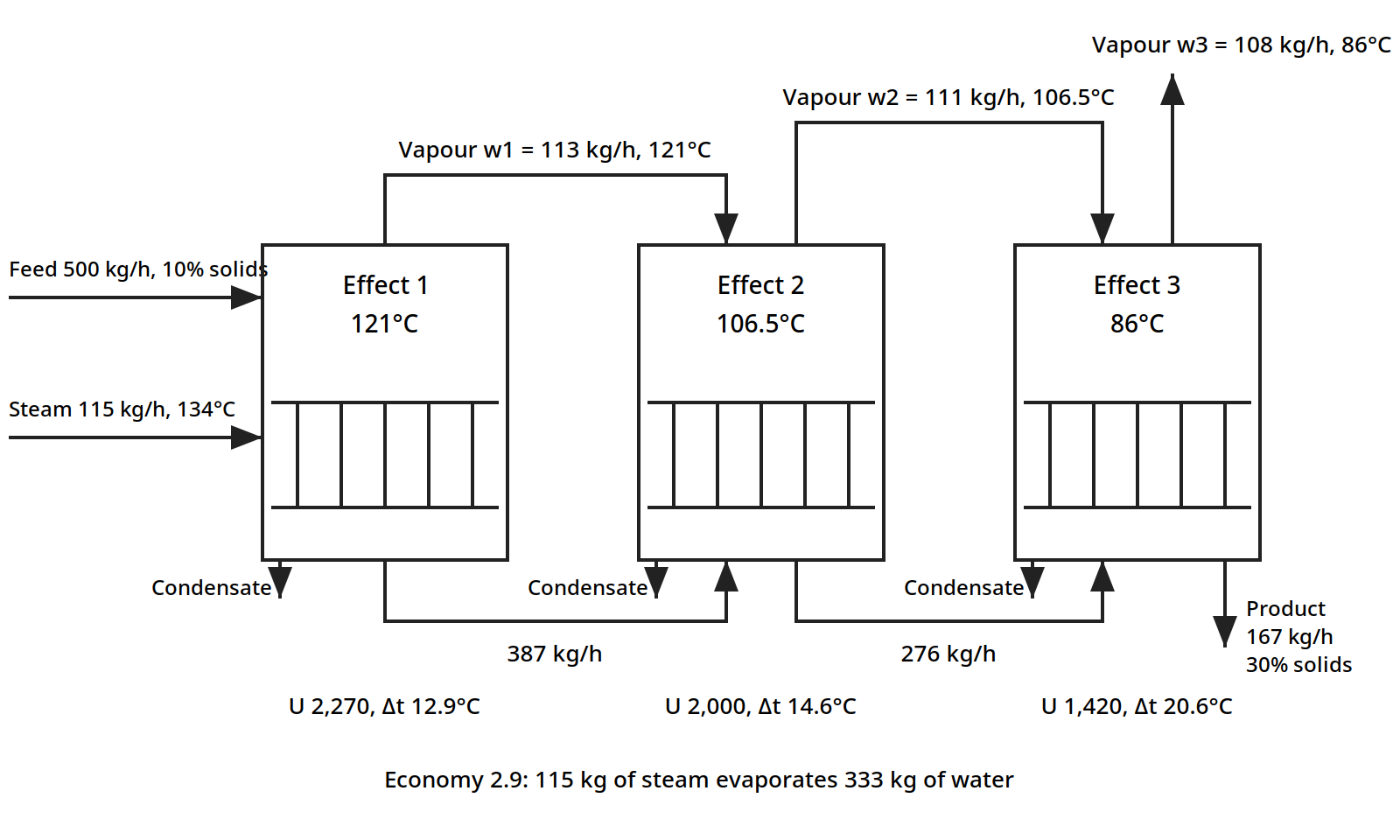
Figure 7.5: Triple effect evaporator for Worked example 7.3 (Earle Example 8.4): three effects in series, forward feed, following the arrangement of Earle Fig. 8.2. All flows and temperatures are the book's.
Mass balance, per hour: feed 500 kg, of which 50 kg is solids and 450 kg is liquid. Product is 50/0.30 = 167 kg, of which 50 kg is solids and 117 kg is liquid. Evaporation is 500 - 167 = 333 kg h⁻¹.
Heat balance: from the steam tables, the condensing temperature of steam at 200 kPa gauge is 134°C and the latent heat is 2,164 kJ kg⁻¹. The evaporating temperature in the final effect under 60 kPa absolute is 86°C, and the latent heat is 2,294 kJ kg⁻¹. Equating the heat transfer in each effect, q₁ = q₂ = q₃, so U₁A₁Δt₁ = U₂A₂Δt₂ = U₃A₃Δt₃, and Δt₁ + Δt₂ + Δt₃ = 134 - 86 = 48°C. With equal areas A₁ = A₂ = A₃, Δt₂ = Δt₁U₁/U₂ and Δt₃ = Δt₁U₁/U₃, so Δt₁(1 + 2,270/2,000 + 2,270/1,420) = 3.73Δt₁ = 48, giving Δt₁ = 12.9°C, Δt₂ = 14.6°C and Δt₃ = 20.6°C. The evaporating temperature in the first effect is 134 - 12.9 = 121°C with a latent heat of 2,200 kJ kg⁻¹, in the second effect 121 - 14.5 = 106.5°C with a latent heat of 2,240 kJ kg⁻¹, and in the third effect 106.5 - 20.6 = 86°C with a latent heat of 2,294 kJ kg⁻¹.
Equating the quantities evaporated in each effect, with w₁, w₂ and w₃ the quantities evaporated in effects 1, 2 and 3, and w_s the steam condensed in effect 1: w₁ x 2,200 = w₂ x 2,240 = w₃ x 2,294 = w_s x 2,164, all in kJ. With w₁ + w₂ + w₃ = 333, solving gives w₁ = 113, w₂ = 111 and w₃ = 108 kg h⁻¹, and w_s = 115 kg h⁻¹. It required 115 kg of steam to evaporate 333 kg of water, which is 0.35 kg of steam per kg of water evaporated, an economy of 2.9. Three effects have nearly tripled the economy of the single effect in Example 7.1, from 0.86 to 2.9.
Table 7.3 shows the same pattern in running costs, from data published in 1954. The steam consumption falls from 1.1 kg per kg of water evaporated with one effect to 0.40 with three, and the total running cost falls to 0.37 of the single effect figure. The gain from the second effect is bigger than the gain from the third, which is the usual pattern: each added effect saves less than the one before, while costing as much to build.
Table 7.3: Steam consumption and running costs of evaporators (Earle Table 8.1)
| Number of effects | Steam consumption (kg steam/kg water evaporated) | Total running cost (relative to a single-effect evaporator) |
|---|---|---|
| One | 1.1 | 1 |
| Two | 0.57 | 0.52 |
| Three | 0.40 | 0.37 |
Table 7.3: Steam consumption and running costs of evaporators. Source: Grosse, H. and Duffield, W. D., 1954, as cited in Earle, Table 8.1, p. 122.
Quick check
Why does a triple effect evaporator use only 0.35 kg of steam per kg of water, when a single effect uses 1.17 kg?
Check your answer
Because the vapour boiled off in the first effect condenses in the second and boils more water there, and the vapour from the second does the same in the third. One kilogram of steam does its work three times over.
7.6 Vapour recompression and the thermal pump
There is another way to reuse the vapour: compress it so that it condenses at a higher temperature, then feed it back as the heating steam. This is vapour recompression, and it can push the economy far above the number of effects, because the same vapour is used again and again.
In mechanical vapour recompression, the vapour is compressed in a compressor, and the work of compression is the energy input instead of fresh steam. The compression is treated as isentropic and read off a Mollier diagram for steam. In thermocompression, a jet of high pressure steam entrains the vapour in a Venturi, and the mixed stream condenses in the heating surface. Ibarz gives the thermocompression balance as Eq. 18.33, from Vián and Ocón, 1967.
The thermal pump is a related idea using two evaporators with a closed heating circuit: the vapour from one evaporator heats the other, and the circuit carries the heat round. Ibarz gives orange juice as the example of a product concentrated this way. The point of all three is the same: the latent heat of the vapour is the biggest energy flow in the plant, and any of it that can be caught and used again is money saved.
7.7 Condensers: getting rid of the vapour
The vapour that is not reused must be condensed, and the condenser is part of the evaporator design. Earle gives two worked examples on the same duty, which show the difference between the two types.
Worked example 7.4: a jet condenser (Earle Example 8.2)
A jet condenser condenses 5,000 kg h⁻¹ of water at a pressure of 20 kPa, corresponding to 15 cm of mercury, with a condensing temperature of 60°C and a latent heat of 2,358 kJ kg⁻¹. Cooling water enters at 18°C and leaves at 35°C at most. The heat removed from the condensate is 2.46 x 10⁶ J kg⁻¹, and the heat taken up by each kg of cooling water is 7.1 x 10⁴ J kg⁻¹. The cooling water needed is 5,000 x 2.46 x 10⁶/7.1 x 10⁴ = 173,000 kg h⁻¹. The cooling water flow is about 35 times the vapour flow: condensing takes a lot of cold water, and the water supply often sets the size of the plant. In a jet condenser the vapour mixes directly with the cooling water, so the two streams leave together.
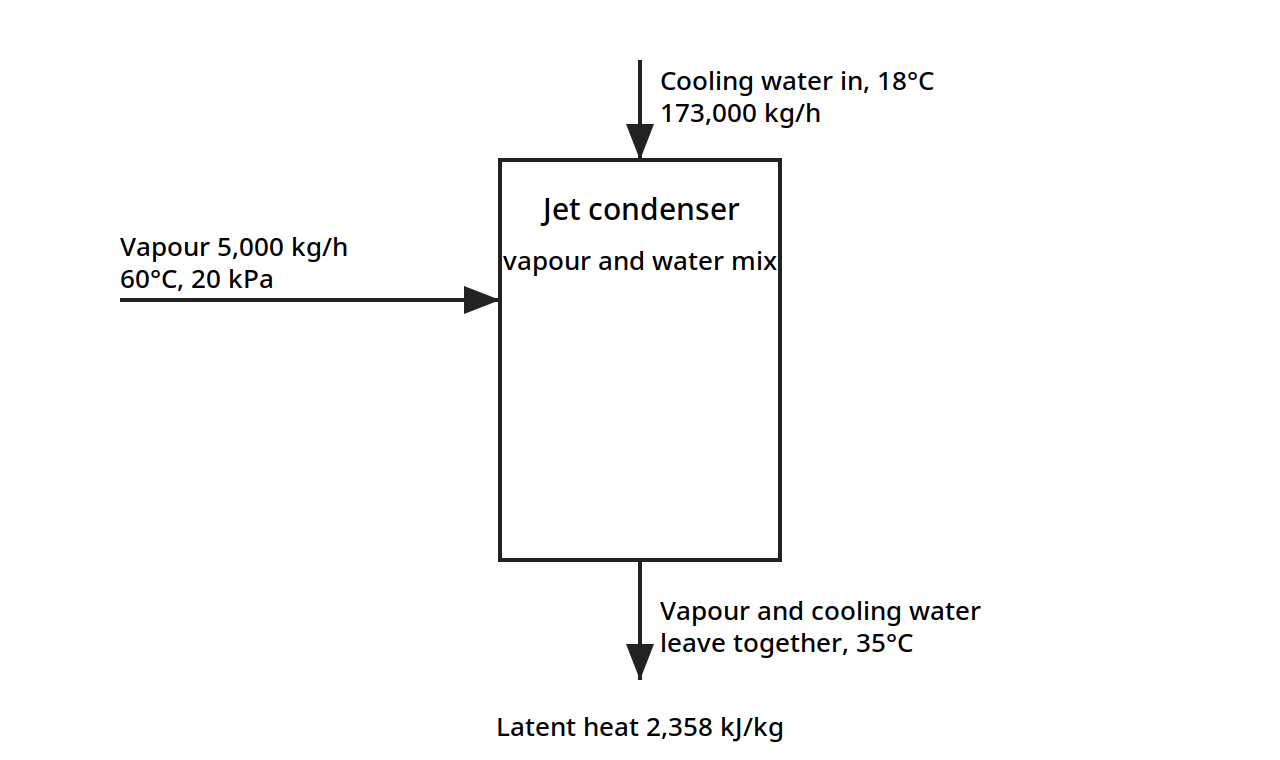
Figure 7.6: Jet condenser for Worked example 7.4 (Earle Example 8.2): the vapour mixes directly with the cooling water, and the two streams leave together. All flows and temperatures are the book's.
Worked example 7.5: a surface condenser (Earle Example 8.3)
The same duty with a surface condenser, where the vapour condenses on tubes and the cooling water stays separate. With U = 2,270 J m⁻² s⁻¹ °C⁻¹ and a mean temperature difference of 33.5°C, the area needed is 45 m². The surface condenser keeps the condensate clean and recoverable, which matters when the condensate is worth keeping, but it costs a heat exchanger and its area.
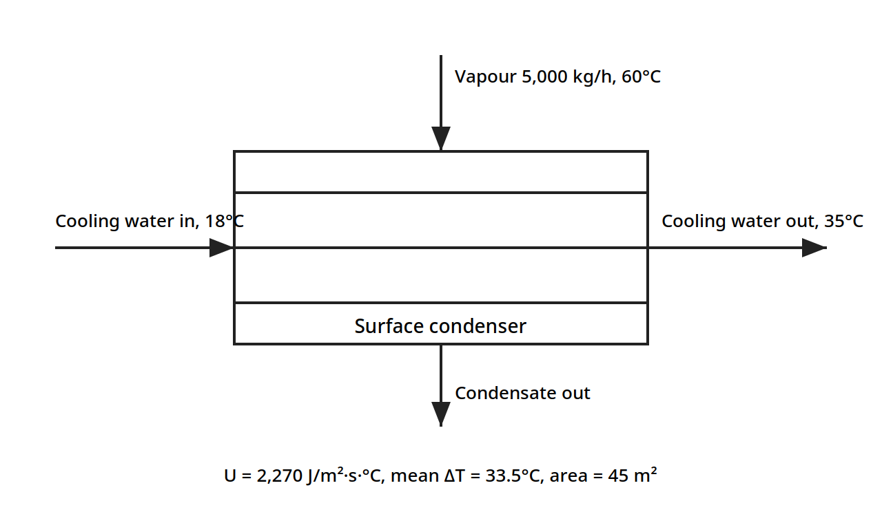
Figure 7.7: Surface condenser for Worked example 7.5 (Earle Example 8.3): the vapour condenses on tubes and the cooling water stays separate. All flows and temperatures are the book's.
7.8 The equipment
Earle's Fig. 8.4 shows three evaporator types side by side: a basket type, a long tube type, and a forced circulation type. The choice between them, and the other types, turns on the liquid: its viscosity, its heat sensitivity, and how much it fouls the tubes.
Open pans are the most elementary form: an open pan in which the liquid is boiled, with heat through a steam jacket or coils, and scrapers or paddles for agitation. They are simple and low in capital cost, but expensive to run because the heat economy is poor.
Horizontal tube evaporators close the pan in, with the heating tubes in a horizontal bundle immersed in the liquid at the bottom of a vertical cylinder. Liquid circulation is rather poor in this type, which limits the heat transfer.
Vertical tube evaporators use vertical tubes so that natural circulation gives good heat transfer. The standard evaporator, shown in Earle's Fig. 8.1, is of this type: recirculation is through a large downcomer, so the liquors rise through the vertical tubes, about 5 to 8 cm in diameter, boil in the space just above the upper tube plate, and recirculate through the downcomers. The hydrostatic head reduces boiling on the lower tubes, which are covered by the circulating liquid. The length to diameter ratio of the tubes is of the order of 15:1. The basket evaporator, Fig. 8.4(a), is a variant of the calandria type in which the steam chest is contained in a basket suspended in the lower part of the evaporator, and recirculation occurs through the annular space round the basket.
Plate evaporators adapt the plate heat exchanger: the spacings between the plates are increased and suitable passages provided so that the much larger volume of the vapours, compared with the liquid, can be accommodated. They give good heat transfer and are easy to clean, which matters for food liquids that foul.
Long tube evaporators use tall slender vertical tubes, with a length to diameter ratio of the order of 100:1, passing vertically upward inside the steam chest. The liquid may pass down through the tubes, a falling film evaporator, or be carried up by the evaporating liquor, a climbing film evaporator. Evaporation occurs on the walls of the tubes. Because circulation rates are high and the surface films are thin, good conditions are obtained for concentrating heat sensitive liquids, with high heat transfer rates and short heating times. The liquid is generally not recirculated, and if sufficient evaporation does not occur in one pass, the liquid is fed to another pass. In the climbing film type, slugs of vapour form as the liquid boils on the inside of the tube, and this vapour carries up the remaining liquid, which continues to boil. Tube diameters are of the order of 2.5 to 5 cm, contact times may be as low as 5 to 10 seconds, and overall heat transfer coefficients may be up to five times as great as from a heated surface immersed in a boiling liquid. In the falling film type the tube diameters are rather greater, about 8 cm, and these are specifically suitable for viscous liquids.
Forced circulation evaporators pump the liquid round the circuit, so the liquid film coefficients can be increased by improving the circulation and the velocity of flow across the heating surfaces. Pumps or impellers can be fitted in the liquid circuit. Using pump circulation, the heat exchange surface can be divorced from the boiling and separating sections, as shown in Fig. 8.4(c). Alternatively, impeller blades may be inserted into flow passages such as the downcomer of a calandria type evaporator. Forced circulation is used particularly with viscous liquids, and it may be worth considering for expensive heat exchange surfaces, where corrosion or hygiene requirements make it pay to get the greatest possible heat flow through each square metre.
Scraped surface and agitated film evaporators come under the heading of forced circulation. In one type the material to be evaporated passes down over the interior walls of a heated cylinder and is scraped by rotating scraper blades to maintain a thin film, high heat transfer and a short and controlled residence time exposed to heat. They are the choice for very viscous liquids and pastes that would not flow through tubes at all.
Evaporation for heat sensitive liquids deserves its own paragraph, because so many food products carry volatile flavour constituents that are lost by long heating. They retain more of these if they are evaporated under conditions favouring short contact times with the hot surfaces: climbing film and falling film evaporators, either tubular or plate types, for solutions of low viscosity, and mechanical transport across heated surfaces, scraped film methods, at higher concentrations and higher viscosities.
Worked example 7.6: a climbing film evaporator for tomato juice (Earle Example 8.6)
Tomato juice at 12% solids is concentrated to 28% solids in a climbing film evaporator 3 m high with a tube 4 cm in diameter. The maximum temperature is 57°C, the feed enters at 57°C, the latent heat is 2,366 kJ kg⁻¹, steam is at 170 kPa gauge, and U = 6,000 J m⁻² s⁻¹ °C⁻¹. What is the rate of evaporation from one tube?
Mass balance, on a basis of 100 kg of feed: feed 100 kg, of which 12 kg is solids and 88 kg is liquid. Product is 12/0.28 = 43 kg, of which 12 kg is solids and 31 kg is liquid. Evaporation is 57 kg per 100 kg of feed.
Heat balance: the area of the evaporator tube is πDH = π x 0.04 x 3 = 0.38 m². The condensing steam temperature at 170 kPa is 115°C from the steam tables. The heat transfer is q = UAΔt = 6,000 x 0.38 x (115 - 57) = 1.32 x 10⁵ J s⁻¹. The heat required per kg of feed for evaporation is 0.57 x 2,366 x 10³ = 1.34 x 10⁶ J. The quantity evaporated is 1.32 x 10⁵/1.34 x 10⁶ = 0.1 kg s⁻¹, so the rate of evaporation is 360 kg h⁻¹ from one tube. A battery of such tubes, each evaporating 360 kg h⁻¹, makes up the industrial evaporator.
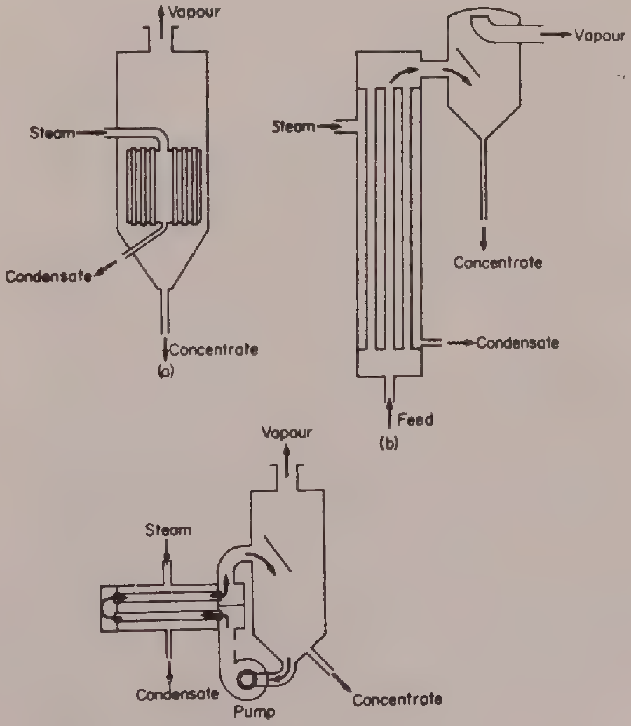
Figure 7.8: Three evaporator types side by side (Earle Fig. 8.4, p. 113): (a) basket, (b) long tube (climbing film), (c) forced circulation. Placed with Worked example 7.6 (Earle Example 8.6).
Try it yourself: feel the boiling point rise
Dissolve as much table salt as you can in a small pan of water, stir until no more dissolves, and bring it to a rolling boil with a thermometer in the liquid. Compare the reading with the boiling point of plain water in the same pan. The salt water will boil a few degrees higher, and that difference is the boiling point rise. Now put a lid on the pan and turn the heat down: the same rise applies at lower pressure, which is why evaporators can run under vacuum and still need to allow for it.
7.9 What the books do and do not give
The books give the single effect balances, the boiling point rise and the Dühring diagrams, the heat transfer coefficients, the multiple effect design with a full worked triple effect example, vapour recompression and the thermal pump, the condenser sizing, and the equipment types with a worked climbing film example. What they do not give is a worked example of vapour recompression with numbers, so the economy of a recompression system cannot be checked against the books alone, and the thermal pump is described without a worked example. The multiple effect example assumes no boiling point elevation and neglects sensible heat, so a real design must add both back in. The cost figures in Table 7.3 come from 1954, and they show the pattern of costs between one, two and three effects, not present day prices. These gaps are stated here so the reader knows where the books stop.
Pause and think: evaporation is where heat transfer, thermodynamics and economics meet in one machine. The steam bill is the biggest running cost, and every improvement, multiple effects, vapour recompression, a better heat transfer coefficient, is a way of getting more water out for the same steam. The cheapest evaporator to build is rarely the cheapest to run.
Key ideas to carry forward
- Evaporation removes water from a liquid by boiling; the solids stay behind and the vapour carries only water.
- Economy is kg of water evaporated per kg of steam used; a good single effect evaporator reaches about 0.86, a triple effect about 2.9.
- The mass balance is set by the solids: feed solids equal product solids, and the evaporation is the difference.
- The heat duty comes from the balances, and the area from Q = UAΔT.
- A solution boils above the boiling point of pure water at the same pressure; the rise grows with concentration and is read from a Dühring diagram.
- The boiling point rise shrinks ΔT, so concentrated solutions need more heating surface.
- The liquid film is usually the biggest resistance to heat transfer; dissolved solids and fouling pull U down.
- Multiple effect evaporation reuses the vapour of one effect as the heating steam of the next, and the economy climbs toward the number of effects.
- Backward feed puts the viscous concentrate at the highest temperature, where it flows best; forward feed is gentler on quality.
- Vapour recompression compresses the vapour and uses it again as heating steam, pushing the economy above the number of effects.
- Condensing takes a lot of cooling water: about 35 times the vapour flow in Example 7.4.
- Climbing film and falling film evaporators give short contact times of 5 to 10 seconds, which protects volatile flavour in heat sensitive liquids.
Glossary
Agitated film evaporator
An evaporator in which a scraper or agitator keeps the liquid as a thin film on a heated surface. Food tech example: concentrating a thick tomato paste that would not flow through tubes.
Backward feed
Feeding a multiple effect evaporator at the last, lowest pressure effect, so the liquid flows against the pressure gradient toward the first effect. Food tech example: concentrating a viscous sugar liquor, where the thickest liquid gets the highest temperature and the lowest viscosity.
Boiling point rise
The amount by which a solution boils above pure water at the same pressure, growing with concentration. Food tech example: saturated salt solution boiling at 109°C at atmospheric pressure, 9°C above water.
Calandria
A vertical tube evaporator in which the tubes sit in a steam chest and the liquid circulates up through the tubes and down through a central downcomer. Food tech example: the standard evaporator for concentrating milk and juice.
Climbing film evaporator
A long tube evaporator in which the liquid is carried up the tubes by the vapour it generates, boiling as it rises. Food tech example: concentrating tomato juice, with contact times of 5 to 10 seconds.
Condenser
A heat exchanger that condenses the vapour from an evaporator, either by mixing it with cooling water, a jet condenser, or on tubes, a surface condenser. Food tech example: the jet condenser in Example 7.4, using 173,000 kg/h of cooling water.
Dühring diagram
A chart plotting the boiling temperature of a solution against the boiling temperature of pure water at the same pressure, with one line per concentration. Food tech example: finding the boiling point of a sucrose solution from the line for 800 g sucrose per 100 g water.
Economy
Kilograms of water evaporated per kilogram of steam used. Food tech example: the triple effect evaporator in Example 7.3, with an economy of 2.9.
Effect
One vessel in a multiple effect evaporator, heated by the vapour of the previous effect. Food tech example: the second effect of a triple effect evaporator, boiling at 106.5°C.
Falling film evaporator
A long tube evaporator in which the liquid flows down the inside of the tubes as a thin film. Food tech example: concentrating viscous fruit puree, using tubes about 8 cm in diameter.
Forced circulation evaporator
An evaporator in which a pump circulates the liquid fast past the heating surface, raising the heat transfer coefficient. Food tech example: concentrating a viscous liquid where natural circulation would be too slow.
Forward feed
Feeding a multiple effect evaporator at the first, highest pressure effect, so the liquid flows with the falling pressure. Food tech example: concentrating a heat sensitive juice, where the product sees the highest temperature only while it is still dilute.
Fouling resistance
The extra resistance to heat transfer from scale deposited on the heating surface. Food tech example: scale on evaporator tubes cutting the overall coefficient, needing cleaning to restore it.
Multiple effect evaporation
Evaporation in several vessels in series, where the vapour from each effect heats the next. Food tech example: a triple effect evaporator concentrating a 10% solution to 30% with 0.35 kg of steam per kg of water.
Overall heat transfer coefficient
The single number U that combines the steam film, tube wall and liquid film resistances, used in Q = UAΔT. Food tech example: U of 1,700 J/m²·s·°C in the single effect evaporator of Example 7.1.
Thermal pump
A system of two evaporators with a closed heating circuit that carries heat between them, reusing vapour heat. Food tech example: concentrating orange juice, as given by Ibarz.
Thermocompression
Recompressing vapour by entraining it in a jet of high pressure steam, so it can be used again as heating steam. Food tech example: a Venturi jet raising low pressure vapour to the pressure of the heating steam.
Vapour recompression
Compressing the vapour from an evaporator so it condenses at a higher temperature and can be used again as heating steam. Food tech example: mechanical recompression with a compressor, using work instead of fresh steam.
References
- Ibarz, A. and Barbosa-Cánovas, G. V. Unit Operations in Food Engineering. CRC Press, 2003. Chapter 18.
- Earle, R. L. Unit Operations in Food Processing. NZIFST, 1983. Chapter 8.
- Brennan, J. G., Butters, J. R., Cowell, N. D. and Lilly, A. E. V. Food Engineering Operations. Applied Science Publishers, 1976. Chapter 11.
- McCabe, W. L. and Smith, J. C. Unit Operations of Chemical Engineering. McGraw-Hill, 1968. Cited for Table 18.2 overall heat transfer coefficients.
- Crapiste, G. H. and Lozano, J. E. Journal of Food Science 53(3), 865-868, 1988. Cited for Table 18.1 Dühring correlation constants.
- Vián, A. and Ocón, J. Elementos de Ingeniería Química. Aguilar, 1967. Cited for Eq. 18.33 thermocompression.
- Grosse, H. and Duffield, W. D. 1954. Cited for Table 8.1 steam consumption and running costs.
Unit 8: Distillation
Note
Unit 8: Distillation
Put a pot of wine on to heat and catch the vapour in a cold tube, and the liquid that drips out is stronger than the wine: the alcohol, which boils lower than water, leaves first and concentrates in the vapour. That is distillation, the oldest separation by boiling point, and it is the only unit operation in this subject that separates two liquids that are already mixed at the molecular level. In food it makes spirits, recovers aromas, strips essential oils from herbs, and takes the fishy taint out of edible oil. This unit follows the vapour up the column, one plate at a time.
Questions to think about
- Why does the vapour above a boiling mixture have a different composition from the liquid?
- What is relative volatility, and why does it decide whether a separation is easy or nearly impossible?
- Why can you never distil ethanol and water to pure ethanol, however many plates you use?
- How does a column with plates turn one boiling into many boilings?
- What do the operating lines on a McCabe-Thiele diagram actually say?
- Why does the feed condition, cold liquid or hot vapour, change the number of plates needed?
8.1 Why distil
Distillation separates liquids by their difference in volatility, by boiling a mixture and condensing the vapour, which is richer in the more volatile component. Earle lists the main food uses plainly: concentrating essential oils, flavours and alcoholic beverages, and deodorization of fats and oils. In each case the separation is between liquids that are mixed together, and no filter or membrane can pull them apart: only the difference in boiling point can.
The operation is expensive in heat, because the whole feed must be boiled, and the vapour must be condensed, and the heat is used once unless it is recovered. That is why distillation is used in food only where the product is worth it: a spirit, a flavour concentrate, an essential oil, or an oil that must be deodorized. The design question is always the same: how many stages of contact between liquid and vapour are needed to reach the wanted purity, and how much reflux must be returned to the top of the column to make those stages work.
Quick check
Why is distillation used for spirits and essential oils, but not for concentrating a sugar solution?
Check your answer
Because distillation separates two volatile liquids by boiling point. Sugar does not evaporate, so it stays behind when water boils off: that separation is evaporation, not distillation.
8.2 Vapour liquid equilibrium: what the vapour holds
Everything in distillation rests on one fact: the vapour above a boiling liquid mixture has a different composition from the liquid, richer in the more volatile component. The equilibrium between the two phases is described by three laws, and the books give all three.
The Gibbs phase rule sets how many variables can be chosen freely: L = C - F + 2 (19.1), where L is the degrees of freedom, C the number of components and F the number of phases. For a binary mixture with two phases, liquid and vapour, L = 2, so fixing the pressure and one composition fixes everything else: the temperature and the other composition follow.
Dalton's law says the partial pressure of a component in the vapour is its mole fraction times the total pressure: pᵢ = yᵢP (19.1), where yᵢ is the mole fraction in the vapour and P the total pressure.
Raoult's law says the partial pressure of a component over an ideal solution is its mole fraction in the liquid times its vapour pressure as a pure liquid at the same temperature: pᵢ = xᵢpᵢ° (19.2). For a binary mixture of A and B, with P = pₐ + p_b, the liquid composition follows as xₐ = (P - p_b°)/(pₐ° - p_b°) (19.6). Raoult's law holds for ideal solutions; real solutions deviate, and the books use activity coefficients where the deviation matters.
Henry's law covers the dilute end: pᵢ = xᵢH (19.3), where H is Henry's constant, the partial pressure proportional to the mole fraction when the component is present in small amounts.
Put Dalton and Raoult together and the equilibrium curve appears: for each liquid composition x, the vapour composition y is fixed, and plotting y against x gives the curve that every distillation design starts from.
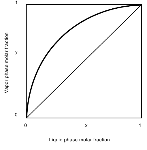
Figure 8.1: Vapour liquid equilibrium diagram. Vapour molar fraction y against liquid molar fraction x, both from 0 to 1. The equilibrium curve sits above the diagonal from (0,0) to (1,1): at every composition the vapour is richer in the more volatile component than the liquid it came from. (Ibarz, Fig. 19.3, p. 674)
The curve sits above the diagonal everywhere, which is the whole reason distillation works: at every liquid composition, the vapour is richer in the volatile component than the liquid. The gap between the curve and the diagonal is the separation gained in one stage of contact. Where the curve hugs the diagonal, the gap is small, the separation per stage is small, and many stages are needed. Where the curve meets the diagonal, at the pure components and at an azeotrope, the gap is zero and no separation is possible at all.
8.3 Relative volatility and the azeotrope
The gap between the curve and the diagonal is measured by the relative volatility, α_AB, the ratio of the volatilities of the two components:
α_AB = [yₐ(1 - xₐ)]/[xₐ(1 - yₐ)] (19.9)
For an ideal system it is the ratio of the pure component vapour pressures, α_AB = pₐ°/p_b°. The equilibrium curve can then be written in one line:
yₐ = α_ABxₐ/[1 + (α_AB - 1)xₐ] (19.10)
When α is large, the curve rises steeply and a few stages give a large separation. When α is close to 1, the curve hugs the diagonal and the separation is hard: the books warn that the McCabe-Thiele method should not be applied when the relative volatility is less than 1.3 or greater than 5, because the design becomes unreliable. If the volatilities at the top and bottom of the column differ by less than 15%, an average α can be used; if they differ by more, the curve must be built in sections.
The limit of the whole operation is the azeotrope, a mixture that boils at a constant composition, so that the vapour has the same composition as the liquid and no further separation is possible by simple distillation. Ethanol and water form a minimum boiling point azeotrope: 89.5 mole% ethanol and 10.5 mole% water, which is 95.6% ethanol and 4.4% water by weight, boiling at 78.15°C. Earle states the consequence plainly: the column limits are 100% water and 95.6% ethanol and 4.4% water, however many stages are used. No number of plates will carry ethanol past 95.6% by weight, because at that composition the equilibrium curve touches the diagonal. Getting past it needs a different operation, such as adding a third component or using a molecular sieve, and the books do not cover those here.
Earle's Fig. 9.10 shows the same fact as a boiling point and concentration diagram, with a liquid composition line and a vapour composition line that meet at the azeotrope. Below the azeotrope the vapour is always richer in alcohol than the liquid, so distillation enriches the alcohol; at the azeotrope the two lines meet and enrichment stops.
Quick check
A mixture has a relative volatility of 1.1. Is this an easy separation or a hard one, and why?
Check your answer
A hard one. The equilibrium curve sits very close to the diagonal, so each stage gains almost nothing, and many stages and a high reflux ratio are needed.
8.4 Simple distillation and flash
The simplest distillation is a single stage: a liquid is partly vaporized, the vapour is condensed, and the two products are separated. The vapour is richer in the volatile component and the remaining liquid is poorer, and that is one stage of separation. Repeating it, boiling the product again, enriches it further, and a batch still does exactly this, boiling the charge and taking off the vapour as it comes, with the composition of the product falling as the charge is depleted.
A flash distillation is the continuous version of one stage: the feed is heated and let down in pressure so that part of it vaporizes, and the vapour and liquid are separated in a flash vessel. The split is fixed by the equilibrium at the flash temperature and pressure, and by the heat balance. One flash gives one stage, and it is used where a rough split is enough, or as the first step before a column.
8.5 Continuous rectification: the column
A rectification column turns one boiling into many by stacking stages, each a plate on which liquid and vapour meet, exchange, and part. The vapour rises, growing richer in the volatile component at each plate; the liquid falls, growing poorer. At the top the vapour is condensed, part is taken off as distillate and part is returned as reflux, which provides the liquid that flows down the column. At the bottom the liquid is boiled in a reboiler, or kettle, and part of the vapour rises back up the column. The column in Ibarz Fig. 19.7 shows the whole arrangement.
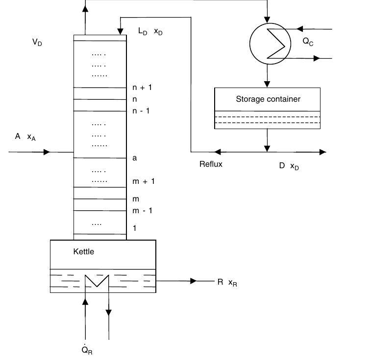
Figure 8.2: Rectification column. Plates are numbered from the top: n + 1, n, n - 1 above the feed plate a, and m + 1, m, m - 1, 1 below it. Feed A with composition xₚ enters at plate a. Vapour Vₙ leaves the top to the condenser, which removes heat Qₕ; part of the condensate is taken as distillate D with composition xₙ and part returns as reflux Lₙ. At the bottom the kettle supplies heat Q̇ₙ and the residue R with composition xₙ leaves. (Ibarz, Fig. 19.7, p. 683)
Earle draws the same column in the form a food plant would recognize: a fractionation column with plates, feed entering at the middle, steam to a boiler at the bottom, a condenser at the top with cooling water, top product drawn from the condenser and bottom product drawn from the boiler. The second half of his figure shows the bubble cap plates themselves: two trays, with vapours rising through bubble caps and liquid flowing across each tray, the contact that makes each plate a stage.
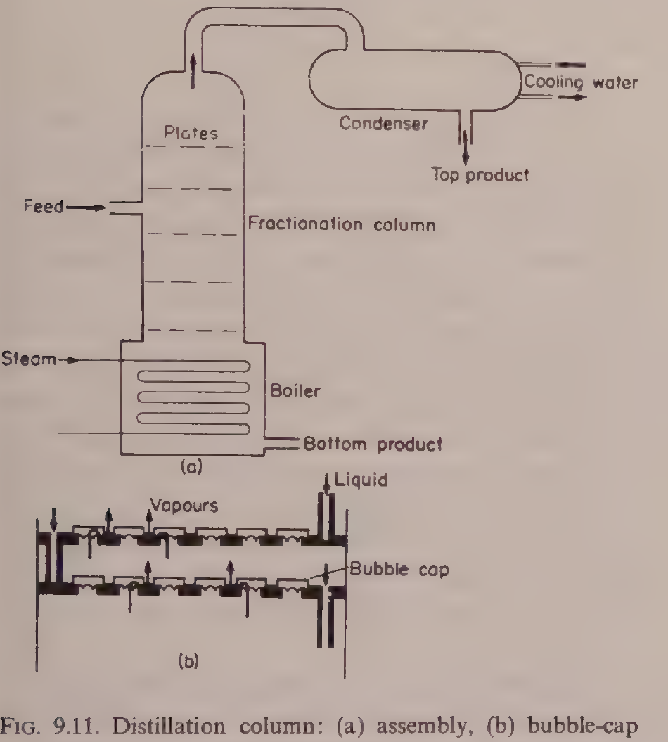
Figure 8.3: (a) Fractionation column with plates, feed at the middle, steam to the boiler at the bottom, condenser at the top with cooling water, top product drawn from the condenser and bottom product drawn from the boiler. (b) Bubble-cap plates: two trays, with vapours rising through bubble caps and liquid flowing across each tray. (Earle, Fig. 9.11, p. 141)
The McCabe-Thiele method
The McCabe-Thiele method finds the number of plates by drawing the separation on the equilibrium diagram. It rests on four hypotheses: the specific heats of the two components are constant and equal, the latent heats are constant and equal, the heats of mixing are zero, and the column is adiabatic. Under those conditions the molar flows of liquid and vapour are constant in each zone of the column, and the operating lines are straight.
The enrichment line, for the section above the feed, is yₙ = (L_D/V_D)xₙ₊₁ + Dx_D/V_D (19.46a), or in terms of the reflux ratio r = L_D/D, yₙ = [r/(r+1)]xₙ₊₁ + x_D/(r+1) (19.46b). It passes through the point (x_D, x_D) on the diagonal and through (0, x_D/(r+1)) on the y axis. The exhaust line, for the section below the feed, is given by Eq. 19.47 and passes through (x_R, x_R) on the diagonal.
The two lines meet at the feed, and where they meet is set by the q-line, which describes the thermal condition of the feed: y = [q/(q-1)]x - xₐ/(q-1) (19.48), passing through (xₐ, xₐ) on the diagonal, with slope m = q/(q-1). The value q is the heat needed to evaporate one mole of feed divided by the molar latent heat. The feed balances are L_m = L_n + qA (19.43) and V_m = V_n + (q-1)A (19.44), where A is the feed flow and the subscripts n and m mark the enrichment and exhaust sections.
Table 8.1: The q-line for different feed conditions (Ibarz, Section 19.5)
| q | Feed condition | Slope m = q/(q-1) |
|---|---|---|
| q > 1 | Subcooled liquid | 1 < m < ∞ |
| q = 1 | Liquid at its bubble point | m = ∞ |
| 0 < q < 1 | Liquid-vapour mixture | ∞ > m > 0 |
| q = 0 | Vapour at its dew point | m = 0 |
| q < 0 | Overheated vapour | 1 > m > 0 |
A cold feed, q > 1, has a q-line sloping steeply upward, and it condenses some vapour in the column, adding liquid to the exhaust section. A feed at its bubble point, q = 1, has a vertical q-line. A feed that is part vapour, 0 < q < 1, has a q-line sloping downward, and a saturated vapour feed, q = 0, has a horizontal q-line. The feed condition moves the intersection of the operating lines, and so moves the number of plates needed.
The construction is drawn in Fig. 8.4. The steps are drawn between the operating lines and the equilibrium curve, starting at the distillate composition (x_D, x_D) and stepping down to the residue composition (x_R, x_R). Each step is one theoretical plate. The book's diagram shows seven steps: 6 full steps plus one small fractional step at the bottom left, counted as a whole stage.
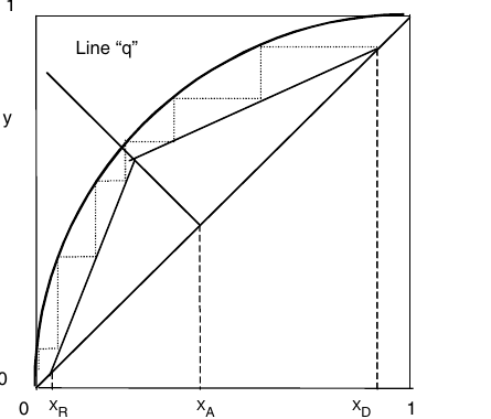
Figure 8.4: McCabe-Thiele diagram. Vapour molar fraction y against liquid molar fraction x, both 0 to 1. The equilibrium curve sits above the diagonal. The q-line slopes down to the right, through the operating-line intersection, to the feed composition xₚ on the diagonal. The enrichment operating line runs from (xₙ, xₙ) to its intersection with the q-line, and the exhaust operating line runs from that intersection to (xₙ, xₙ). Dashed verticals mark xₙ, xₚ and xₙ. The steps between the operating lines and the equilibrium curve, drawn dotted, start at (xₙ, xₙ) and number 7 as printed: 6 full steps plus one small fractional step, counted as a whole stage. (Ibarz, Fig. 19.9, p. 690)
The diagram is read from the top down. Each horizontal step runs from an operating line to the equilibrium curve, giving the vapour leaving a plate; each vertical step runs from the equilibrium curve down to the operating line, giving the liquid leaving the next plate down. Counting the steps gives the number of theoretical plates. The feed plate is the step that crosses the intersection of the two operating lines.
Reflux: minimum, operating and total
The reflux ratio r = L_D/D is the lever that sets the slope of the enrichment line and so the number of plates. At total reflux, all the condensed vapour is returned and no distillate is taken: the operating line becomes the diagonal y = x, the steps are as wide as they can be, and the number of plates is the minimum. The Fenske equation gives that minimum directly:
N + 1 = log[((xₐ/x_b)_D)((x_b/xₐ)_R)]/log α_AB (19.53)
where the subscripts D and R mark the distillate and the residue.
At minimum reflux, the operating lines just touch the equilibrium curve, and the number of plates becomes infinite: the separation is possible but never finished. The minimum reflux ratio is found from the intersection of the q-line with the equilibrium curve. For a bubble point feed, r_m = (x_D - yₐ*)/(yₐ* - xₐ) (19.50), where yₐ* is the vapour in equilibrium with the feed; for a dew point feed, r_m = (x_D - xₐ)/(xₐ - xₐ*) (19.51); and in general r_m = (x_D - yₐ*)/(yₐ* - xₐ*) (19.49). A real column runs between the two extremes, with a reflux ratio above the minimum and a plate count above the Fenske minimum. The books warn that the McCabe-Thiele method should not be applied when the reflux ratio is less than 1.1 times the minimum, or when more than 25 plates are needed, because the design becomes unreliable.
The Fenske-Underwood equation, Eq. 19.52, extends the Fenske result to a finite reflux ratio, giving the minimum number of plates at a given reflux. In practice the designer picks a reflux ratio, often 1.2 to 1.5 times the minimum, and counts the plates off the diagram.
Quick check
What happens to the number of plates if the reflux ratio is raised?
Check your answer
It falls. A higher reflux ratio steepens the enrichment line toward the diagonal, widening the steps, so fewer plates reach the wanted separation, at the cost of more heat in the reboiler and more cooling in the condenser.
8.6 From theoretical plates to a real column
The McCabe-Thiele diagram counts theoretical plates, stages where the leaving liquid and vapour are in equilibrium. A real plate is never that good: the contact is imperfect, some vapour bypasses the liquid, and the liquid may not mix fully. The gap is measured by the plate efficiency.
The global efficiency is η = N_TS/N_RS x 100 (19.56), the number of theoretical stages divided by the number of real stages, or η = (N_TS - 1)/(N_RS - 1) x 100 (19.57) when the kettle is counted as one stage. Plate columns in food and chemical service commonly run at 20 to 80% efficiency, so a column needing 10 theoretical plates may need 15 to 50 real plates.
The Murphree efficiency measures a single plate. The vapour efficiency is η_MV = (yₙ - yₙ₋₁)/(yₙ* - yₙ₋₁) x 100 (19.58), where yₙ* is the vapour that would be in equilibrium with the liquid leaving the plate. The liquid efficiency is η_ML = (xₙ₊₁ - xₙ)/(xₙ₊₁ - xₙ*) x 100 (19.59). A Murphree efficiency can exceed 100% on a real plate, which is a sign that the vapour and liquid on the plate are not uniform, and that the simple stage model is only an approximation.
Column diameter
The diameter is set by the vapour velocity: too fast, and liquid is carried up the column, flooding it; too slow, and the vapour does not bubble properly through the liquid on the plates. The Souders-Brown equation gives the flooding velocity:
v_FLO = K√[(ρ_L - ρ_G)/ρ_G] (19.60)
where ρ_L and ρ_G are the liquid and vapour densities and K is a constant read from Fig. 19.14, from King, 1980, which depends on the plate spacing and the liquid flow. The design velocity is a fraction of the flooding velocity, and the diameter follows from the vapour flow and the velocity. The books give the method; the value of K must be read from the chart for the plate spacing chosen.
Multiple feeds and side draws
A column can take more than one feed, at different plates, and can draw off a product from the side as well as the top and bottom. Ibarz treats these in Figs. 19.12 and 19.13, with the balances in Eqs. 19.54 and 19.55. Each feed has its own q-line, and each draw changes the flows in the section below it, so the operating lines change slope at each feed and each draw. The principle is the same as for a single feed: draw the equilibrium curve, draw the operating lines section by section, and count the steps. A side draw is used when a middle component is wanted as a product, or when a feed of intermediate composition can be taken off without going to the top or the bottom.
Discontinuous rectification
A batch still with a column on top, run as a discontinuous rectification, can be operated in two ways: holding the distillate composition constant by raising the reflux ratio as the charge is depleted, or holding the reflux ratio constant and letting the distillate composition fall. The first gives a uniform product and a rising heat load; the second gives a falling product quality and a steady operation. Small food stills, for essential oils and spirits, are usually run the first way, taking a cut of the best product and then a second cut at lower strength.
Steam distillation
Steam distillation is the form of distillation most used for essential oils and flavours, and Ibarz gives it its own section, 19.6. Live steam is blown through the material, and the steam carries the volatile oil with it, even though the oil itself boils far above 100°C. The oil and the water are immiscible, so each exerts its own vapour pressure, and the mixture boils when the sum of the two vapour pressures reaches the total pressure, which happens below 100°C at atmospheric pressure. The oil is recovered by condensing the mixed vapour and separating the oil from the water. The product never sees a high temperature, which is why steam distillation is used for delicate aromas that would be destroyed by direct boiling.
Try it yourself: see the steps in a kitchen still
Put a little red wine in a saucepan, cover it with an upturned metal bowl, and put ice on top of the bowl. Warm the wine gently, never boiling it hard. Vapour rises, condenses on the cold bowl, and drips into a small cup set in the middle of the pan. Smell the liquid in the cup and compare it with the wine: it is stronger and sharper, because the vapour was richer in alcohol than the liquid. That is one stage of distillation. A column does the same thing many times over, plate after plate.
8.7 Worked example: enriching alcohol in one stage (Earle Example 9.13)
This is the book's own food distillation worked example, a single stage continuous distillation enriching an alcohol and water mixture. A feed of 12% alcohol is distilled so that 25% of the feed leaves as top product. At 95.5°C, a liquid containing 1.9 mole% alcohol is in equilibrium with a vapour containing 17 mole% alcohol.
First the feed is changed to mole fractions. The molecular weights are 46 for alcohol and 18 for water, so
x_F = (12/46)/(88/18 + 12/46) = 0.05
The operating equation for the stage, from the mass balance with 25% of the feed leaving as top product, is 4 x 0.05 = 3x + y, where x is the mole fraction of alcohol in the liquid leaving and y is the mole fraction in the vapour. The equilibrium relation at 95.5°C is x = (1.9/17)y. Solving the two together gives y = 0.15 mole fraction. Changing back to weight, the product from the still is 31% alcohol.
One stage has taken a 12% feed to a 31% product. The same arithmetic, repeated plate by plate up the column, is the McCabe-Thiele construction of section 8.5, and it is what carries the alcohol toward the 95.6% azeotrope limit, and no further.
Figure 8.3, repeated here with Worked example 8.7 (Earle Example 9.13): the fractionation column of Earle Fig. 9.11.
8.8 What the books do and do not give
This must be stated plainly, because the coverage is thin. Ibarz Chapter 19 gives the equilibrium theory, the relative volatility, the column balances, the McCabe-Thiele construction, the q-line, the reflux limits, the Fenske equation, the efficiencies, the column diameter, multiple feeds and side draws, discontinuous rectification and steam distillation, but it gives no worked examples at all, only end of chapter problems with no answers printed. Earle gives a short distillation section with the food uses, the ethanol water azeotrope, the boiling point and concentration diagram, and one worked example, Example 9.13, the single stage alcohol enrichment above. There is no worked example in either book of a full McCabe-Thiele design with numbers, no worked example of a food distillation beyond the single stage alcohol example, and no worked example of steam distillation with numbers. The azeotrope limit, the plate efficiency range and the single stage example are the book's own facts, and they are given above as printed. Nothing has been invented to fill the gaps.
Pause and think: distillation is the most powerful separation in this subject and the most limited. It can split two liquids that nothing else can touch, plate by plate, but it stops dead at the azeotrope, and every plate costs heat. The art is knowing when the separation is worth the steam, and when a simpler operation will do.
Key ideas to carry forward
- The vapour above a boiling mixture is richer in the more volatile component than the liquid: that gap is what distillation exploits.
- The Gibbs phase rule says a binary two phase system has two degrees of freedom: fixing pressure and one composition fixes the rest.
- Dalton's law, Raoult's law and Henry's law together give the equilibrium curve of y against x.
- Relative volatility α measures how easy the separation is: near 1 it is hard, large it is easy, and the books warn against using McCabe-Thiele below 1.3 or above 5.
- An azeotrope boils at constant composition, so the vapour and liquid are the same and no further separation is possible: ethanol and water stop at 95.6% by weight, boiling at 78.15°C.
- A rectification column stacks plates, each one a stage of contact between rising vapour and falling liquid, with reflux returned at the top and a reboiler at the bottom.
- The McCabe-Thiele diagram counts theoretical plates by stepping between the operating lines and the equilibrium curve, starting at the distillate composition.
- The q-line sets where the enrichment and exhaust lines meet, and it depends on the feed condition: cold liquid, bubble point liquid, mixed feed, dew point vapour, or superheated vapour.
- Total reflux gives the minimum plates, by the Fenske equation; minimum reflux needs infinite plates. A real column runs between the two.
- Real plates are 20 to 80% efficient, so a real column needs more plates than the diagram counts.
- The column diameter is set by the flooding velocity, from the Souders-Brown equation.
- Steam distillation carries a volatile oil with steam at a temperature below 100°C, which protects delicate aromas.
- One stage took a 12% alcohol feed to a 31% product in Earle's Example 9.13; the column repeats that step plate by plate.
Glossary
Azeotrope
A mixture that boils at a constant composition, so the vapour has the same composition as the liquid and distillation cannot separate it further. Food tech example: ethanol and water at 95.6% ethanol by weight, boiling at 78.15°C.
Bubble cap plate
A column plate with caps that force the rising vapour to bubble through the liquid flowing across the tray. Food tech example: the trays in Earle's Fig. 9.11, where vapour rises through the caps and liquid flows across.
Bubble point
The temperature at which a liquid first starts to boil at a given pressure. Food tech example: a feed at its bubble point has q = 1 and a vertical q-line.
Dew point
The temperature at which a vapour first starts to condense at a given pressure. Food tech example: a feed of vapour at its dew point has q = 0 and a horizontal q-line.
Distillate
The product taken from the top of a distillation column, rich in the volatile component. Food tech example: the spirit drawn from the condenser of a still.
Enrichment section
The part of a column above the feed plate, where the vapour is enriched in the volatile component. Food tech example: the plates n + 1, n and n - 1 in Ibarz Fig. 19.7.
Equilibrium curve
The curve of vapour composition y against liquid composition x at equilibrium, sitting above the diagonal. Food tech example: the curve in Fig. 8.1, which shows that the vapour is always richer in the volatile component than the liquid.
Exhaust section
The part of a column below the feed plate, where the volatile component is stripped from the falling liquid. Food tech example: the plates m + 1, m, m - 1 and 1 in Ibarz Fig. 19.7.
Flash distillation
A single stage continuous distillation in which a heated feed is let down in pressure so part of it vaporizes, and the vapour and liquid are separated. Food tech example: a first rough split of a mixture before it enters a column.
Flooding
The condition in a column when the vapour velocity is so high that liquid is carried upward, and the column stops working properly. Food tech example: the limit set by the Souders-Brown equation, Eq. 19.60.
Minimum reflux ratio
The lowest reflux ratio at which a separation is possible, needing an infinite number of plates. Food tech example: the reflux ratio at which the operating lines just touch the equilibrium curve.
Murphree efficiency
The efficiency of a single plate, measured by how close the vapour leaving it comes to equilibrium with the liquid leaving it. Food tech example: a plate with a vapour Murphree efficiency of 70%, meaning the vapour achieves 70% of the change to equilibrium.
Operating line
A straight line on the McCabe-Thiele diagram relating the vapour leaving a plate to the liquid entering it, one for the enrichment section and one for the exhaust section. Food tech example: the enrichment line from (x_D, x_D) in Fig. 8.4.
q-line
The line on the McCabe-Thiele diagram that shows the thermal condition of the feed and sets where the two operating lines meet. Food tech example: a vertical q-line for a feed at its bubble point, q = 1.
Reboiler
The heater at the bottom of a column that boils the liquid and sends vapour back up the column. Food tech example: the kettle in Ibarz Fig. 19.7, supplying heat Q with a dot above it.
Rectification
Continuous distillation in a column with plates, reflux and a reboiler, giving a sharp separation. Food tech example: a fractionation column separating alcohol from water toward the azeotrope.
Reflux ratio
The ratio of liquid returned to the top of the column to distillate taken off, r = L_D/D. Food tech example: raising the reflux ratio cuts the number of plates needed but raises the heat load.
Relative volatility
The ratio of the volatilities of two components, α_AB, which measures how easy they are to separate by distillation. Food tech example: a mixture with α of 1.1 is hard to separate, needing many plates.
Residue
The product taken from the bottom of a distillation column, poor in the volatile component. Food tech example: the water rich bottom product of an alcohol column.
Steam distillation
Distillation in which live steam carries a volatile component, such as an essential oil, out of a material at a temperature below 100°C. Food tech example: recovering essential oil from herbs without destroying the aroma by direct boiling.
Theoretical plate
An ideal stage in which the leaving liquid and vapour are in equilibrium. Food tech example: one step on the McCabe-Thiele diagram, with a real plate achieving only 20 to 80% of it.
Total reflux
Running a column with all the condensed vapour returned and no distillate taken, giving the minimum number of plates. Food tech example: the condition where the operating line is the diagonal y = x.
References
- Ibarz, A. and Barbosa-Cánovas, G. V. Unit Operations in Food Engineering. CRC Press, 2003. Chapter 19.
- Earle, R. L. Unit Operations in Food Processing. NZIFST, 1983. Chapter 9.
- King, C. J. Separation Processes. McGraw-Hill, 1980. Cited for Fig. 19.14, the Souders-Brown flooding constant.
- Vián, A. and Ocón, J. Elementos de Ingeniería Química. Aguilar, 1967. Cited in Ibarz Chapter 19.
Unit 9: Extraction, Expression and Adsorption
Note
Unit 9: Extraction, Expression and Adsorption
A spoonful of ground coffee meets hot water, and a few minutes later the water is brown, fragrant and full of flavour, while the grounds left behind are pale and spent. Nothing was cut, nothing was burned, and no new chemical was made. A liquid simply carried something out of a solid. The same quiet move, repeated on a factory scale, gives us cooking oil from seed, sugar from beet, and the clear juice in a bottle. How does a liquid pull one thing out of a solid and leave the rest behind, and how does a maker get almost all of it out without drowning the factory in solvent? This unit follows that question from a single coffee ground to a countercurrent extractor.
Questions to think about
- What is the difference between the solid that is left behind, the liquid that does the work, and the liquid that comes out carrying the goods?
- Why does crushing the solid, heating the liquid and stirring the mixture all speed up an extraction?
- How can a triangular diagram show three things at once, and what does the curve inside it mean?
- Why does a maker use several stages instead of one big tank, and why does the solvent run the opposite way to the solid?
- When is it better to squeeze a solid than to wash it with a solvent?
- How does a bed of black granules take the bitter taste out of orange juice without taking the juice itself?
9.1 What extraction is: a liquid that carries one thing away
Solid-liquid extraction is the transfer of a soluble part, the solute, from a solid into a liquid, the solvent. The solid that stays behind is called the inert solid, because it does not dissolve. The liquid that comes out, carrying the solute, is the extract, also called the overflow or the miscella. The wet solid that is left, still holding some solution in its pores, is the underflow, also called the exhausted solid or the raffinate in some books.
The books use several names for the same move. Lixiviation, washing, percolation and leaching all describe a solvent passing over or through a solid and carrying a solute away. Washing is the name used when the solid is the product and the solute is an impurity to be removed, as in washing lactose out of cheese curd. Extraction is the name used when the solute is the product, as in taking oil out of seed. The engineering is the same in both cases.
Food gives plenty of examples. Vegetable and animal oils are taken from seed, nut and fish tissue. Sugar is taken from beet and cane. Tea and coffee give their soluble solids to hot water. Fruit and spice extracts, pectin from exhausted fruit pulp, and the bitter compound limonene taken out of orange juice all use the same idea. In every case the maker wants the same three things: get as much solute out as possible, use as little solvent as possible, and keep the extract as strong as possible.
Quick check
Name the three streams that leave an extraction stage, and say which one carries the solute out as product.
Check your answer
The overflow (extract or miscella) carries the solute out as product, the underflow is the exhausted wet solid, and the solvent is the liquid fed in to do the work.
9.2 The three stages inside every extraction, and which one is slowest
Ibarz describes extraction as three stages that follow one another. First, the solute dissolves the moment the solvent touches it: an instantaneous dissolution at the solid surface. Second, the dissolved solute diffuses through the pores of the solid toward the outside, following Fick law in the form N_S = -D_L dC/dz, where N_S is the solute flux, D_L is the diffusivity in the liquid, and dC/dz is the concentration gradient inside the pore. Third, the solute crosses from the particle surface into the bulk liquid, at a rate N_S = (1/A) dM/dt = K_L (C_S - C), where A is the particle surface, M is the mass transferred, K_L is the mass transfer coefficient, C_S is the concentration at the surface, and C is the concentration in the bulk liquid.
The slowest stage controls the whole operation, and in most food extractions that stage is the diffusion inside the pores. That is why the practical rules of extraction all point the same way. Crush the solid into smaller particles, and the diffusion path gets shorter. Raise the temperature, and the diffusivity rises while the viscosity falls. Stir the mixture, and the transfer coefficient K_L at the surface rises. Use a solvent that likes the solute and flows easily, and the solute moves faster. None of these changes the chemistry: they all shorten the slowest step.
The solvent itself must be chosen with care. It should dissolve the solute well and leave the rest of the solid alone, so the extraction is selective. It should have a low viscosity, so it flows through the solid bed and drains away cleanly. It should be easy to take away from the extract afterwards, usually by evaporation, and it must be safe in food use. Ibarz lists hexane, heptane, cyclohexane, benzene, trichloroethylene and carbon disulfide as solvents named in the older literature for vegetable oils. The book itself notes the limits: trichloroethylene is toxic and its use is limited, and benzene brings health problems. In modern food practice the common choice for oilseeds is hexane, used with care and removed afterwards, and the book gives a paprika example in which the final oleoresin holds less than 10 ppm of hexane.
Quick check
A maker grinds the feed finer and the extraction speeds up. Which stage did the grinding shorten, and why?
Check your answer
It shortened the diffusion of solute through the pores of the solid, because the distance the solute must travel to reach the particle surface is smaller.
9.3 Overflow, underflow and retention: the triangular diagram
To design an extraction, the maker needs to know how much solution the exhausted solid holds on to. That quantity is the retention, r, in kg of solution retained per kg of inert solid. The underflow leaving a stage is a mixture of inert solid and retained solution, and the solution it retains has the same composition as the overflow leaving that stage, because the two streams are in equilibrium. The inert solid itself never appears in the overflow, so the mass fraction of inert solid in the overflow, Y_I, is 0.
Ibarz plots these mixtures on a triangular diagram, a right triangle in which the vertex of the right angle is the inert component I, and the other two vertices are the solvent D and the solute S. The mass fraction of solute is read on the horizontal axis, X_S, and the mass fraction of solvent on the vertical axis, X_D. The mass fraction of inert solid follows from the difference of one minus the sum of the other two. The hypotenuse of the triangle is the overflow, because every point on it holds no inert solid. The underflow points sit on a curve inside the triangle, the retention curve, which runs from a point G on the vertical axis to a point K near the base.
Three lines in the diagram carry the whole design. Curve (a) is the retention curve itself, the real behaviour of the solid. Line (b) is the line of constant retention of solution: it runs from G to a point H on the base, and it says the solid always holds the same total mass of solution, whatever the solute concentration. Line (c) is the line of constant retention of solvent: it runs from G to the vertex S, and it says the solid always holds the same mass of solvent. A real solid may follow either line, or a curve between them, and the book gives the equations for both. For constant retention of solution, X_D = r/(r + 1) - X_S. For constant retention of solvent, X_D = r/(r + 1) (1 - X_S). The tie lines that join an overflow point on the hypotenuse to its underflow point on the retention curve all pass through the inert vertex I, which is how the diagram is read in practice.
Right triangle with the inert component I at the right angle, solvent D at the top and solute S at the bottom right. Curve (a) is the retention curve from G to K, line (b) is constant retention of solution from G to H, line (c) is constant retention of solvent from G to S. The hypotenuse D to S is the overflow.
Figure 9.1: Triangular diagram for solid-liquid extraction: (a) retention curve, (b) constant retention of solution, (c) constant retention of solvent. (Ibarz, Fig. 21.1, p. 777.) The retention curve carries no numeric coordinates in the book, so its path in this drawing follows the printed shape; all vertices, axes, points G, H and K, and lines (a), (b) and (c) are as the book gives them.
Quick check
A point sits on the hypotenuse of the triangular diagram. How much inert solid does that stream hold, and what is it called?
Check your answer
None: the mass fraction of inert solid is 0 on the hypotenuse, and the stream is the overflow, or extract.
9.4 The rectangular diagram: the same facts without the inert solid
When the inert solid is left out of the picture, the same mixtures can be plotted on a rectangular diagram, with the axes free of inert solid. Ibarz defines N = X_I / (X_S + X_D), the inert solid per unit of solution, and X' = X_S / (X_S + X_D), the solute fraction in the solution on an inert-free basis, with Y' = Y_S / (Y_S + Y_D) for the overflow. On this diagram the overflow line is the abscissa itself, because N = 0 for the overflow, and the underflow points sit on a curve above it. The two diagrams say the same thing in different shapes: the triangular diagram keeps the inert solid in view, the rectangular diagram hides it so the solution compositions are easier to read. A maker uses whichever one suits the calculation at hand.
9.5 One stage: balances, the pole, and the least solvent that can work
A single stage is a box with four streams: the feed R_A comes in, fresh solvent D comes in, the underflow R_1 goes out, and the overflow E_1 goes out. The overall balance is R_A + D = R_1 + E_1 = M, where M is the pole, the mixture point of feed and solvent. The solute and solvent balances fix where M sits, and the tie line through M gives the compositions of R_1 and E_1. The book gives the pole coordinates as X_SM = (R_A X_SRA + D Y_SD) / (R_A + D) and X_DM = (R_A X_DRA + D Y_DD) / (R_A + D).
There is a smallest amount of solvent that can do the job at all, D_MIN. It is found when the pole M sits exactly on the retention curve. In that case the underflow R_1 coincides with M, the distance R_1M is 0, and the overflow E_1 is 0: no extract comes out. So a real plant must always work with more solvent than the minimum, and the minimum is a limit to design against, not a flow to run at.
Figure 9.2: Single-stage system: (a) scheme of the contact, (b) operation on the triangular diagram. (Ibarz, Fig. 21.5, p. 783.) The retention curve in (b) carries no numeric coordinates in the book, so its path follows the printed shape; all points, lines and labels are as the book gives them.
9.6 Several stages: running the streams against each other
One stage rarely gets enough solute out, so plants use several stages. In a concurrent system the fresh solvent is split between the stages, and Ibarz shows the best yield comes when the solvent is split equally, D_i = D_T / n, where D_T is the total solvent and n is the number of stages. In a countercurrent system the solid and the solvent move in opposite directions: fresh solvent meets the most exhausted solid last, and the strongest extract leaves beside the fresh feed. The overall balance is R_A + E_{n+1} = R_n + E_1 = M, and the stages are stepped off with a pole P given by R_A - E_1 = R_i - E_{i+1} = P. The minimum solvent in a countercurrent system is found when the final overflow is in equilibrium with the feed, or when the final underflow is in equilibrium with the solvent, whichever comes first.
Countercurrent working is the reason a factory extractor can be both strong and thrifty. The fresh solvent, which has the most power to dissolve, meets the solid that has the least solute left, so it squeezes out the last of it. The strong extract, already carrying solute, meets the fresh feed, which has plenty of solute to give, so the extract leaves as strong as the feed can make it. The solvent use stays low and the extract stays strong, which is the pair of aims set out in section 9.1.
Quick check
In a countercurrent extractor, which stream does the fresh solvent meet first: the fresh feed or the most exhausted solid?
Check your answer
The most exhausted solid. Fresh solvent meets the solid with the least solute left, and the strongest extract leaves beside the fresh feed.
9.7 Worked examples from Earle: oil from soya, and washing curd
Example 9.6: oil from soya beans. Oil is to be extracted from soya beans in a countercurrent stage-contact apparatus using hexane. The initial oil content of the beans is 18%, the final extract solution is to contain 40% of oil, and 90% of the total oil is to be extracted. The oil is extracted from the beans in the first mixer, equilibrium is reached in each stage, and the crushed bean solids in the underflow retain half their weight of solution after each settling stage. How many contact stages are necessary?
Basis: 100 kg of raw beans. In 100 kg there are 82 kg of bean solids and 18 kg of oil. In the final underflow, 82 kg of beans retain 41 kg of solution, and that solution holds 10% of the oil, that is 1.8 kg, so 16.2 kg of oil go into the final overflow. The extract holds 16.2 kg of oil and 24.3 kg of solvent, a total of 40.5 kg, and the total solvent entering is 63.5 kg.
Working stage by stage from the balances, with x as the oil fraction in the underflow and y as the oil fraction in the overflow, the book finds x_1 = 0.4 and y_2 = 0.23 after the first stage, y_4 = 0.049 after the third stage, and y_5 = 0.00315 after the fourth stage. The required terminal condition is that the underflow from the final stage holds less than 1.8 kg of oil, that is x_n less than 1.8 / 41 = 0.044. Since y_5 = 0.00315 is less than 0.044, four stages of contact are sufficient.
The same result comes from the McCabe-Thiele graphical method. For all stages after the first, the operating line is y_{n+1} = 0.646 x_n - 0.028, and the equilibrium line is y_n = x_n, because the retained solution has the same concentration as the overflow. Stepping off between the two lines from the entry conditions gives the same answer: three steps are not sufficient, four are.
Example 9.7: washing lactose out of casein curd. Washing is almost identical to extraction, except the solid is the product and the solute is an impurity to be removed, and the solvent is water, which is cheap and readily available. A curd has a liquid content of 66% and that liquid holds 4.5% lactose. Calculate the residual lactose in the casein after drying if the curd is washed three times with 194 kg of fresh water each time, and calculate the water that would be needed in a single wash to reach the same lactose content. Assume perfect washing and draining of the curd to 66% moisture each time.
100 kg of curd hold 66 kg of solution, and the 66 kg hold 4.5%, that is 3 kg of lactose. In the first wash, (194 + 66) = 260 kg of solution hold 3 kg of lactose, so the 66 kg of solution left after draining hold (66 / 260) x 3 = 0.76 kg. After the second wash the lactose left is (66 / 260) x 0.76 = 0.19 kg. After the third wash it is (66 / 260) x 0.19 = 0.048 kg. After washing and drying, 0.048 kg of lactose remain with 34 kg of dry casein, so the lactose content of the product is 0.048 / 34.05 = 0.14%, using 3 x 194 = 582 kg of wash water.
To reach 0.048 kg in one wash would need x kg of water, where (3 x 66) / (x + 66) = 0.048, giving x = 4060 kg. Three small washes use 582 kg of water to do what one big wash would need 4060 kg to do. That is the whole case for staging, in one pair of numbers.
The general rules behind the example are the washing equations. After n washings, x_n = x [1 / (1 + y)]^n, equation 9.11. If the same total quantity of water is used all in one stage, the impurity content is x = x [1 / (n y + 1)], equation 9.12. Splitting the water always wins.
Quick check
A curd is washed twice with the same water each time. Does the second wash remove the same mass of lactose as the first?
Check your answer
No. Each wash removes the same fraction of what is left, so the mass removed falls each time: 3 kg falls to 0.76 kg, then to 0.19 kg in this example.
9.8 The Ibarz chapter problems: the same method, worked through
Ibarz gives no worked examples inside the text of Chapter 21. It gives end-of-chapter problems with solutions, and this section states their results plainly as chapter problems, not as worked examples from the text.
Problem 21.1: flour and oil, one stage. 500 kg of flour holding 10% oil are treated with 3000 kg of solvent in a single stage, with a retention of 0.8 kg of solution per kg of inert solid. The retention line is X_D = 0.444 - X_S, the pole M sits at X_SM = 0.014 and X_DM = 0.857, the underflow leaves at X_S = 0.007 and X_D = 0.437, and the overflow leaves at Y_S = 0.016 and Y_D = 0.984. The underflow is R_1 = 813.2 kg and the overflow is E_1 = 2686.8 kg. The oil extracted is 44.1 kg, which is 88% of the oil in the flour.
Figure 9.5: Graphical method to obtain underflow and overflow concentrations (Ibarz Fig. 21.P1, p. 812), for Problem 21.1.
Problem 21.2: fish flour, three concurrent stages. Fish flour holding 38% oil is treated at 1000 kg/h with 750 kg of ether per stage in three concurrent stages, with a retention that rises with the oil fraction in the overflow, r = 0.6 + 0.3 y_S + 7 y_S^2. The book reads the stage compositions from the triangular diagram: stage 1 gives underflow X_SR1 = 0.21 and overflow Y_SE1 = 0.34, with E_1 = 96.2 kg/h and R_1 = 1653.8 kg/h; stage 2 gives X_SR2 = 0.10 and Y_SE2 = 0.20, with E_2 = 1069.2 kg/h and R_2 = 1334.6 kg/h; stage 3 gives X_SR3 = 0.04 and Y_SE3 = 0.10, with E_3 = 834.6 kg/h and R_3 = 1250 kg/h. The combined extract holds Y_SE = 0.165, the oil recovered is 330 kg/h, and the yield is 86.84%.
Figure 9.6: Graphical solution of Problem 21.2 (Ibarz Fig. 21.P2, p. 815).
Problem 21.3: cod liver oil, countercurrent. Cod liver oil is extracted so that 90% is recovered and the overflow holds 60% oil, with a retention r = 2 / 3.2 = 0.625. On a basis of 100 kg, the feed holds X_SRA = 0.251 and X_IRA = 0.749, the final underflow is R_n = 121.85 kg at X_SRn = 0.021, X_DRn = 0.364 and X_IRn = 0.615, the first overflow is E_1 = 37.65 kg, and the solvent feed is E_{n+1} = 59.5 kg. The retention line is X_D = 0.385 - X_S, the pole P sits at (0.04, -0.242), and the graphical construction gives 6 theoretical stages.
Figure 9.7: Graphical calculation of theoretical stages (Ibarz Fig. 21.P3, p. 818), for Problem 21.3.
Problem 21.4: soluble coffee, countercurrent. Soluble coffee is made at 3000 kg/h from beans holding 24% soluble solids, with 5% of the solute left in the final underflow, an overflow of 35% solids, and a retention of 1.6 kg of solution per kg of inert solid. The book finds E_1 = 1954.3 kg/h, R_n = 5928 kg/h, and a water requirement of E_{n+1} = 4882.3 kg/h. The retention line is X_D = 0.615 - X_S, the pole P sits at (0.034, -1.215), and the construction gives 9 theoretical stages, or 12 real stages at 75% stage efficiency.
Figure 9.8: Graphical calculation of theoretical stages (Ibarz Fig. 21.P4, p. 821), for Problem 21.4.
9.9 Equipment: from a laboratory flask to a factory extractor
Batch percolators are the simplest factory form: a vessel with a false bottom, filled with the solid, through which solvent is passed until the extract is strong enough, then drained. A diffusion battery is a set of such vessels connected so the solvent passes from one to the next, and the freshest solvent always meets the most exhausted solid: a countercurrent system built from batch vessels. The Robert diffusion battery works this way for sugar beet.
Continuous extractors move the solid instead of the solvent. The Bollman extractor, also called the Hansa-Muehle extractor, is a tall vertical bucket elevator: perforated buckets carry the solid up one side and down the other, fresh solvent sprays on the solid near the top, half miscella is collected part way down and sprayed again, and the final miscella leaves at the bottom.
Figure 9.3: Bollman extractor. (Ibarz, Fig. 21.11, p. 802.) All tanks, streams and labels are as the book gives them.
Other continuous forms named in the book are the Hildebrandt U immersion extractor, in which a screw carries the solid up one leg while solvent flows the other way; the Bonotto vertical column; the Rotocel, a rotating carousel of cells; the vertical immersion column; and the C.M.B. percolation extractor and the De Smet extractor. The choice between them turns on the solid: how it flows, how it packs, how fine it is, and how much solvent it holds.
The Soxhlet extractor is the laboratory form, and it shows the idea in its purest shape. Solvent boils in the cauldron, condenses in the condenser, drips onto the solid in the extractor, and when the extractor fills to the top of the siphon, the whole charge siphons back into the cauldron. The same solvent is used again and again, each time carrying a little more solute into the cauldron, until the solid is exhausted. It is slow and small, but it is the standard way to measure how much extractable matter a solid holds.
Figure 9.4: Soxhlet extractor. (Ibarz, Fig. 21.17, p. 807.) The left half is the book's labelled scheme; the right half is the book's detailed drawing of the glass apparatus.
9.10 Expression: squeezing instead of dissolving
Expression takes the liquid out by pressure instead of by a solvent. The liquid is pressed out of the solid matrix, and the solid left behind is a cake. Brennan gives the presses used in food plants. A hydraulic plate press works at 2 to 4 tons per square inch, in thin layers, with the pressure raised gradually so the liquid has time to escape. A cage press holds the material in a perforated cylinder with drainage strings that give the liquid a path out. A roller press, with grooved rollers, is the form used for sugar cane. A screw press, or expeller, drives the material along a shaft turning at 5 to 500 rpm, building barrel pressures of 20,000 to 40,000 psi, with throughputs up to 200 tons in 24 hours and a residual cake holding 4 to 5% liquid.
How well expression works turns on four things: the yield stress of the solid, the porosity of the cake, the viscosity of the liquid, and the compressive force applied. A soft fruit pulp gives up its juice under a gentle press. An oilseed needs an expeller. A material that forms a tight, low-porosity cake holds its liquid back whatever the pressure. Expression is the right choice where the liquid is already there and only needs to be pushed out; extraction is the right choice where the solute is locked inside the solid and a solvent must go in and fetch it. Many plants use both: press first to take the free liquid, then extract the pressed cake to take the rest.
Quick check
A maker presses an oilseed and the cake still holds 5% liquid. Would a second press, or a solvent extraction of the cake, recover more of that liquid?
Check your answer
A solvent extraction of the cake. Pressing has reached its limit for that cake, and a solvent can dissolve out the oil that pressure alone cannot push out.
9.11 Adsorption and ion exchange: catching molecules on a surface
Adsorption is the catching of a substance, the adsorbate, on the surface of a solid, the adsorbent. The adsorbent is usually a porous solid with a very large internal surface: activated carbon and molecular sieves are the common examples. In physical adsorption the molecules are held by Van der Waals forces, the binding is weak, and the process is reversible: the adsorbate can be taken off again. In chemisorption the binding happens at active points on the surface and is stronger. Electric forces can also play a part. Ion exchange is a related operation in which ions in a liquid are swapped for ions held on a resin: cationic resins swap cations and anionic resins swap anions, and the uses include desalination and water conditioning.
Food uses are mostly about taking something unwanted out of a liquid. The bitter compound limonene is taken out of orange juice on polymer adsorbents. Brown colour compounds, melanins and melanoidins, are taken out of clarified juice on activated carbon. The adsorbent must catch the unwanted molecule and let the wanted ones pass, which is why the choice of adsorbent and the isotherm matter so much.
The equilibrium between a liquid and an adsorbent is described by an isotherm, a curve of the amount adsorbed against the concentration left in the liquid. The Langmuir isotherm is m_A / m_0 = K C_A / (1 + K C_A), where m_A is the mass adsorbed, m_0 is the saturation mass, C_A is the concentration in the liquid, and K is a constant. The Freundlich isotherm is m_A = K (C_A)^n. The BET isotherm extends the idea to several layers of molecules. The ion exchange separation factor is K = (1 - Y) X / [Y (1 - X)], with Y = C_A / C_A0 and X = E_A / E_M, where E_A is the amount of ion A on the resin and E_M is the total exchange capacity.
Kinetics follow the same pattern as extraction: transfer from the bulk liquid to the surface, N = k_F (C - C_i), then diffusion inside the particle, then the adsorption step itself. In most cases the first stage, the transfer to the surface, controls the rate.
Stage operation is drawn on an m-C diagram, amount adsorbed against concentration. For a single contact the operating line is m_S = -(F/S) C_S + (m_E + (F/S) C_E), with a slope of -F/S, where F is the liquid flow and S is the adsorbent flow. Repeated simple contact steps down the isotherm stage by stage. In a countercurrent moving bed the operating line has slope F/S, and there is a maximum (F/S)_MAX, found by the tangent to the isotherm: past it, the operating line crosses the isotherm and the separation fails. A fixed-bed column is described by a moving exchange zone: the breakpoint is taken at 5% of the inlet concentration and saturation at 95%, the zone height is z_C, the column volume to the breakpoint is V_C = V_T - V_R, the mass retained is M_R = V_R C_0, and the times are t_C = V_C / q and t_T = V_T / q. For a symmetrical breakthrough curve the factor i is 0.5 and the formation time is t_F = 0.5 t_C. For adsorption the zone height is z_C = (F A / (K' k_F a_S)) ln 19 for C_1 = 0.05 C_0 and C_2 = 0.95 C_0, and for ion exchange z_C = (F A / (k_F a_S)) ((K + 1) / (K - 1)) ln 19. Wilke gives the empirical form z_C = b v^0.51, with b = 37.4 for Ca2+ and Mg2+ exchanged by Na+.
9.12 Adsorption worked examples from the Ibarz chapter problems
These are end-of-chapter problems with book solutions, stated plainly as such.
Problem 22.1: taking the brown colour out of clarified juice. A clarified juice has a browning value A420 of 0.646, and activated carbon is dosed at b = 0 to 0.26 kg of carbon per kg of solution, with equilibrium m values of 11.4, 7.75, 4.35, 2.98 and 1.79. In repeated contact with 0.025 kg of carbon per kg of juice, the operating line has slope -L/S = -40, and five stages bring the juice from A420 0.646 down to 0.200, through stage values 0.470, 0.365, 0.285, 0.225 and 0.180. In a countercurrent moving bed, (L/S)_MAX = 25.11, so the minimum carbon is 39.82 kg, and the operating carbon for 1000 kg/h of juice is 79.64 kg.
Figure 9.9: Graphical calculation of the stages and maximum slope, and the movable column (Ibarz Fig. 22.P1, p. 848), for Problem 22.1.
Problem 22.2: limonene out of orange juice. Orange juice holds 110 ppm of limonene and flows at 100 kg/h through a column of 0.15 m2 cross section, with adsorbent of density 950 kg/m3, a transfer coefficient of 1.5 x 10^2 h-1, a capacity of 10 mg/kg, and an isotherm m = 0.12 C, with symmetrical breakthrough. The book finds the exchange zone height z_C = 0.0646 m, the bed height 3.12 m, and the breakpoint at 25 min.
Figure 9.10: Conditions of an exchange zone (Ibarz Fig. 22.P2, p. 850), for Problem 22.2.
Problem 22.3: softening water by ion exchange. Water flows at 8000 kg/h holding magnesium salts at 40 meq/kg, through a resin of capacity 15 eq/kg, a separation factor of 50, an apparent density of 550 kg/m3, and a column 30 cm in diameter, with K_L a_S = 2.5 x 10^6 l/(h.m3) = 2500 h-1, and symmetrical breakthrough. The book gives z_C = 0.139 m, V_C = 0.00981 m3, a breakpoint of 1.046 h, which is 63 min, a saturation time of 1.298 h, which is 78 min, and a magnesium content of 32 meq/kg after 75 min of operation.
Figure 9.11: Single contact: (a) operation sketch; (b) operation in the equilibrium diagram (Ibarz Fig. 22.2, p. 830), for Problem 22.3.
One inconsistency in the book must be stated plainly. The problem statement says the column contains 110 kg of resin, but the calculation that follows uses 25 kg: V_RESIN = 25 kg / 550 kg/m3 = 0.04546 m3, giving a total column height of z = 0.643 m and a saturation volume V_S = V - V_C = 0.03565 m3. Every downstream number follows from 25 kg, so the 110 kg in the statement reads as a misprint, and this unit follows the calculation as printed.
Quick check
A fixed-bed column is run until the outlet reaches 5% of the inlet concentration. What is that moment called, and what does it mean for the bed?
Check your answer
It is the breakpoint. It means the exchange zone has reached the end of the bed and the unwanted substance is starting to escape, so the bed is nearly spent.
9.13 Food applications: sugar, coffee, tea, oils and juice
Sugar beet is washed and sliced, then extracted with hot water in a diffusion battery to give an extract holding about 15% dissolved solids. The extract is purified by sedimentation and filtration, concentrated, and the sugar is crystallised out by centrifuge. The same countercurrent idea, water running against the solid, serves a commodity made in millions of tonnes.
Instant coffee is roasted and crushed beans extracted with water. The final solution holds 25 to 30% solids, and it is then atomised to give instant coffee grains. The solid just charged is extracted with water at 100 C, and as the process goes on the temperature of the water is increased. High temperatures favour the hydrolysis of insoluble carbohydrates, which become soluble and raise the soluble solids content of the final solution. But very high temperatures can hydrolyse substances that give undesirable aromas and flavours to the extract, so the temperature is a balance between yield and quality.
Instant tea is extracted with water at 70 C in the first stages, rising to 90 C in the last, giving an extract of 2.5 to 5% solids. The volatile aroma compounds are distilled off first, the extract is vacuum evaporated to 25 to 50% soluble solids, the aroma is added back, and the concentrate is freeze dried or atomised.
Vegetable oils are extracted with solvents, then the solvent is evaporated off and the oil refined. Paprika oleoresin is extracted to 99.25% oleoresin, and the final product holds less than 10 ppm of hexane, using a volume of solvent of 5 to 10% of the paprika. Fish oil and fish flour, pectin from exhausted fruit pulp, and flavour liquors made with ethanol all use the same operations at different scales.
9.14 What the books do not give
The books used for this unit give no table specific to extraction, so this unit invents none. Ibarz gives no worked examples inside the text of Chapters 21 and 22, only end-of-chapter problems, and those are labelled as such wherever they appear above. Earle gives two worked extraction examples, 9.6 and 9.7, and two worked membrane examples in Unit 10. The FPE proceedings papers listed in the outline for this unit, Emch on extraction of fruit and vegetables and Schwartzberg and colleagues on expression of water and juices in plants, are supplementary papers, and no numbers from them are quoted here because the chapter text already carries the design material. The Desai and Schwartzberg paper on mathematical modelling of leaching processes is listed in the outline with its PDF page not yet located, so it is not cited here.
Try it yourself: Make a cup of tea with one tea bag and a fixed amount of hot water, and time how long the colour takes to reach a shade you like. Then make a second cup with the same bag cut open and the leaves spread loose in the water. Compare the two cups at the same time. The loose leaves colour the water faster, because the diffusion path is shorter and the surface is larger. Then pour a third cup through the used leaves with fresh hot water: the second wash is paler, because each wash takes the same fraction of what is left. That is sections 9.2 and 9.7, in a kitchen.
Key ideas to carry forward
- Extraction moves a solute from a solid into a solvent. The overflow, or miscella, carries the product out, and the underflow is the exhausted solid holding retained solution.
- The slowest stage usually controls the rate, and it is usually diffusion inside the pores, so crushing, heating and stirring all speed the work up.
- Retention, r, is the kg of solution held per kg of inert solid, and the triangular diagram plots the underflow on its retention curve and the overflow on its hypotenuse.
- The pole M fixes a single stage, and the minimum solvent is found when M sits on the retention curve, at which point no overflow comes out.
- Countercurrent stages run the solvent against the solid, so fresh solvent meets the most exhausted solid and the strongest extract leaves beside the fresh feed.
- Three small washes beat one big wash: 582 kg of water in three washes does the work of 4060 kg in one, for the casein curd in Example 9.7.
- Four stages of countercurrent contact take 90% of the oil from soya beans at 40% extract strength, in Example 9.6.
- The Bollman extractor is a bucket elevator that carries the solid past the solvent, and the Soxhlet extractor reuses the same solvent through boiling, condensing and siphoning.
- Expression squeezes the liquid out by pressure. A screw press can reach 20,000 to 40,000 psi and leave a cake holding 4 to 5% liquid.
- Adsorption catches unwanted molecules on a porous solid. Activated carbon takes brown colour from juice, and polymers take bitter limonene from orange juice.
- Adsorption equilibrium follows Langmuir, Freundlich or BET isotherms, and a fixed bed is judged by its breakpoint at 5% of the inlet concentration and its saturation at 95%.
- In Ibarz Problem 22.3 the statement says 110 kg of resin while the calculation uses 25 kg, and this unit follows the calculation as printed.
Glossary
Extraction
The transfer of a soluble part from a solid into a liquid solvent. Food tech example: taking oil out of soya beans with hexane in a countercurrent extractor.
Solute
The soluble part that is taken out of the solid. Food tech example: the oil dissolved out of soya beans, or the soluble solids dissolved out of roasted coffee beans.
Solvent
The liquid that dissolves the solute and carries it out of the solid. Food tech example: hot water as the solvent for instant coffee, or hexane as the solvent for vegetable oil.
Inert solid
The part of the solid that does not dissolve and stays behind. Food tech example: the bean solids left after the oil has been extracted from soya beans.
Overflow
The liquid stream leaving an extraction stage carrying the solute, also called the extract or the miscella. Food tech example: the 40% oil extract leaving the first stage of the soya bean plant.
Underflow
The wet solid leaving an extraction stage, holding retained solution in its pores. Food tech example: the exhausted beet pulp leaving a diffusion battery.
Miscella
The mixture of solvent and dissolved solute that is the product of an extraction, especially in oilseed work. Food tech example: the half miscella collected part way down a Bollman extractor and sprayed again.
Retention
The mass of solution held by the exhausted solid, in kg of solution per kg of inert solid. Food tech example: a retention of 0.8 kg per kg for flour in Ibarz Problem 21.1.
Triangular diagram
A right-angled diagram that plots the solute, solvent and inert solid fractions of extraction mixtures, with the overflow on the hypotenuse and the underflow on the retention curve. Food tech example: reading the underflow and overflow compositions for a single stage from Figure 9.1.
Pole
The mixture point of two streams on a triangular diagram, used to step off the stages of an extraction. Food tech example: the pole M of feed and solvent in a single stage, or the pole P of a countercurrent system.
Countercurrent
An arrangement in which two streams flow in opposite directions, so the freshest of one meets the most exhausted of the other. Food tech example: fresh water meeting the most exhausted beet pulp in a diffusion battery.
Percolation
Passing a solvent down through a bed of solid so it trickles through and extracts as it goes. Food tech example: solvent percolating through a bed of crushed oilseed in a batch percolator.
Expression
Taking liquid out of a solid by pressure instead of by a solvent. Food tech example: a screw press taking oil from seed and leaving a cake holding 4 to 5% liquid.
Expeller
A screw press that drives material along a shaft and squeezes the liquid out under high pressure. Food tech example: an expeller running at up to 200 tons of seed in 24 hours.
Adsorption
The catching of molecules from a liquid or gas on the surface of a porous solid. Food tech example: activated carbon catching brown colour compounds from clarified juice.
Adsorbate
The substance caught on the surface of an adsorbent. Food tech example: limonene caught on a polymer adsorbent from orange juice.
Adsorbent
The porous solid that catches molecules on its surface. Food tech example: activated carbon used to decolourise juice.
Isotherm
A curve showing how much is adsorbed at equilibrium for each concentration left in the liquid, at a fixed temperature. Food tech example: the Langmuir isotherm for a solute on activated carbon.
Ion exchange
Swapping ions between a liquid and a resin that holds ions on its surface. Food tech example: swapping magnesium and calcium ions for sodium ions to soften water.
Breakpoint
The moment when the outlet of a fixed-bed column reaches 5% of the inlet concentration, showing the bed is nearly spent. Food tech example: the 63 minute breakpoint in the water softening column of Ibarz Problem 22.3.
Exchange zone
The band inside a fixed-bed column where the transfer is actually happening, between the saturated part above and the fresh part below. Food tech example: the 0.139 m exchange zone in the water softening column.
References
- Ibarz, A., and Barbosa-Canovas, G. V., Unit Operations in Food Engineering, CRC Press, 2003. Chapter 21, Solid-Liquid Extraction, including Figures 21.1, 21.5, 21.11 and 21.17 and Problems 21.1 to 21.4; Chapter 22, Adsorption and Ionic Exchange, including Problems 22.1 to 22.3.
- Earle, R. L., Unit Operations in Food Processing, 2nd edition, Pergamon Press, 1983. Chapter 9, Contact-Equilibrium Separation Processes, extraction and washing section, including Examples 9.6 and 9.7 and equations 9.11 and 9.12.
- Brennan, J. G., Butters, J. R., Cowell, N. D., and Lilly, A. E. V., Food Engineering Operations, Elsevier, 1969. Chapter 6, Filtration and Expression, Section 6.4, Expression.
Unit 10: Membrane Separation
Note
Unit 10: Membrane Separation
A jug of apple juice is pressed, and the juice that comes out is cloudy. Pass it through a fine enough skin, and the cloud stays behind while clear juice comes through, with no heat and no boiling at all. The same trick, pushed harder, takes salt out of sea water and takes most of the water out of whey, leaving the protein behind. A membrane is a barrier that lets some things through and stops others, and the only power it needs is pressure. How does a thin skin sort molecules by size, and what sets the limit on how fast it can work? This unit follows that question from a juice filter to a reverse osmosis plant.
Questions to think about
- What decides whether a particle passes a membrane or is stopped by it: its size, its charge, or something else?
- Why does water flow from a weak solution into a strong one on its own, and what happens when you push back?
- Why does a membrane that starts fast often slow down, and what is the layer that forms on its surface?
- How can a maker concentrate whey protein twelve times without heating the whey?
- Why does raising the pressure sometimes stop helping, and what does temperature do to the flow?
10.1 Sorting by size: four processes on one scale
A membrane separation needs little energy compared with other separations, because nothing is boiled and nothing changes phase. The feed flows along one side of the membrane, part of it passes through as the permeate, and the rest stays behind as the reject, also called the retentate or the concentrate. The split is made by size, and sometimes by charge, and the four main processes sit on one scale of particle size.
Microfiltration stops suspension particles: the cloud in a juice, yeast cells, fine solids. Ultrafiltration stops macromolecules: proteins, pectin, large gums. Nanofiltration stops sugars and other small organic molecules. Reverse osmosis stops salts, and only water passes. Each step down the scale needs a tighter membrane and a higher pressure, and the drawing below shows the idea: each kind of particle travels down until it meets the membrane that stops it, and only water travels the whole way.
Figure 10.1: Classification of the membrane processes. (Ibarz, Fig. 10.1, p. 266; adapted from Cheryan, 1986.) The symbol shapes follow the book: hexagons for suspension particles, triangles for macromolecules, circles for sugars, squares for salts.
Quick check
A membrane stops proteins but lets sugars and salts through. Which process is it, and what has it kept back?
Check your answer
Ultrafiltration. It has kept back the macromolecules, the proteins, and let the smaller sugars and salts pass into the permeate.
10.2 The basic stage: feed, permeate and reject
Every membrane unit, whatever its shape, is the same box with three streams. The feed F comes in at concentration C_0. The permeate P comes out through the membrane at concentration C_P. The reject S stays behind at concentration C_S. The membrane itself is a thin barrier between the two sides, and the split is described by three numbers. The retention is R = (C_C - C_P) / C_C = 1 - C_P / C_C, equation 10.1, where C_C is the concentration on the feed side. A retention of 1 means nothing of that substance passes; a retention of 0 means it passes freely. The concentration factor is F_C = C_S / C_F, how much stronger the reject has become. The recovery is Q = P / F, how much of the feed has been taken as permeate.
In ultrafiltration the retention is often quoted as a molecular weight cut-off: the molecular weight above which most molecules are retained. Ibarz warns that the cut-off alone is not enough, because a membrane also retains some molecules below the cut-off. When a cut-off value is given, the percentage of molecules of lower molecular weight that are also rejected should be stated beside it.
Feed enters at the top left, the large particles stay above the membrane and leave as reject, and the small particles pass through the membrane and leave as permeate at the bottom right.
Figure 10.2: Basic unit of separation by membrane. (Ibarz, Fig. 10.2, p. 266.)
10.3 Osmosis and reverse osmosis: pushing water uphill
Osmosis was first described by Nollet in 1748, from experiments with wine held in animal stomach containers standing in water. Put a concentrated solution and a dilute solution on the two sides of a semipermeable membrane, and the solvent moves on its own from the dilute side to the concentrated side. The flow raises the level on the concentrated side, and the pressure that builds up is the osmotic pressure. The van't Hoff equation gives it as pi = i C R T, equation 10.4, where C is the molar concentration, R is the gas constant, T is the absolute temperature, and i counts the ions a solute splits into.
Reverse osmosis turns that flow around. Apply a pressure on the concentrated side that is higher than the osmotic pressure, and the solvent flows the other way, from the concentrated side to the dilute side. The drawing below shows both cases: in (a) the water flows into the concentrated solution and the level rises; in (b) a pressure is applied on the concentrated side and the water flows out into the dilute solution.
(a) Osmosis: water flows into the concentrated solution and the level rises. (b) Reverse osmosis: pressure applied on the concentrated side pushes water out into the dilute solution.
Figure 10.3: Scheme of osmosis (a) and reverse osmosis (b). (Ibarz, Fig. 10.3, p. 268.)
How strong the push needs to be depends on the food. Table 10.1 gives the osmotic pressure of food fluids at room temperature, from Cheryan's Ultrafiltration Handbook of 1986. A 1% salt solution already needs 862 kPa to hold back, milk at 9% nonfat solids needs 690 kPa, apple juice at 15% total solids needs 2070 kPa, and a coffee extract at 28% total solids needs 3450 kPa. The stronger the food, the harder the push, and that sets the pressure a reverse osmosis plant must reach before a single drop comes through.
Table 10.1: Osmotic pressure of certain food fluids at room temperature (Ibarz Table 10.1, from Cheryan, 1986)
| Food fluid | Osmotic pressure (kPa) |
|---|---|
| Lactic acid, 1% w/v | 552 |
| Coffee extract, 28% total solids | 3450 |
| Sodium chloride, 1% w/v | 862 |
| Lactose, 5% w/v | 380 |
| Milk, 9% nonfat solids | 690 |
| Whey, 6% total solids | 690 |
| Apple juice, 15% total solids | 2070 |
| Orange juice, 11% total solids | 1587 |
| Grape juice, 16% total solids | 2070 |
Table 10.1: Osmotic pressure of certain food fluids at room temperature. (Ibarz, Table 10.1, p. 287.)
Quick check
Apple juice at 15% solids has an osmotic pressure of 2070 kPa. What happens if a reverse osmosis plant applies only 1500 kPa to it?
Check your answer
Nothing comes through in the reverse direction. The applied pressure is below the osmotic pressure, so water still flows by osmosis into the juice instead of out of it.
10.4 The layer that forms on the membrane: concentration polarization
The flow through a membrane happens in stages: from the solution to the membrane wall, into the membrane, through its layers, and out from the wall to the dilute liquid. Ibarz lists those four stages, then adds a fifth that appears in real operation: a polarization layer forms at the wall, because solute piles up there faster than it can diffuse back into the bulk liquid. The polarization factor is F_P = C_m / C_C, the concentration at the membrane wall over the concentration in the bulk.
That layer does three kinds of harm. It raises the osmotic pressure at the wall, so the driving force falls and the flux drops. It can make solute precipitate on the surface. And it can block the pores. Stirring the feed, or running it in turbulent flow, thins the layer but never removes it fully. The hydraulic model of the layer gives C_m = C_P + (C_C - C_P) exp(J / k_S), equation 10.13, where J is the flux and k_S = D_S / delta_p is the mass transfer coefficient through the polarization layer of thickness delta_p. The coefficient is found from the Colburn analogy, (Sh) = j_H (Re)(Sc)^(1/3), equation 10.15, with the Colburn factor j_H = 0.023 (Re)^-0.2 for laminar flow (Re below 2100), equation 10.16, and j_H = 1.86 (Re)^-2/3 (d_e / l_c)^1/3 for turbulent flow (Re above 10^4), equation 10.17. The diffusivity of the solute comes from the Wilke-Chang equation, D_S = 7.4 x 10^-8 T (psi M)^1/2 / [eta (V bar_m)^0.6], equation 10.18, where psi is the association parameter of the solvent, 2.6 for pure water, and V bar_m is the molar volume of the solute at its boiling temperature.
The geometry of the module sets the numbers in those equations. Table 10.2 gives the characteristic geometric parameters for the common reverse osmosis module shapes, and Table 10.3 gives the molecular volumes used in the Wilke-Chang calculation, from Perry and Chilton's Chemical Engineer's Handbook of 1982.
Table 10.2: Characteristic geometric parameters of reverse osmosis modules for flat, spiral, and tubular configurations (Ibarz Table 10.2, from Lombardi and Moresi, 1987)
| Configuration | a | A_m | d_e | l_c | l_pd | l_pc |
|---|---|---|---|---|---|---|
| Flat, annular | (pi / 2) (R_e - R_i) | pi (R_e^2 - R_i^2) | 2 h | (R_e - R_i) | (R_e - R_i) | 70 d_e |
| Flat, rectangular | H h | H L | 2 h | L | L | 70 d_e |
| Spiral | H h | H L / N | 2 h | L | L / N | 0 |
| Tubular | (pi / 4) D_i^2 | pi D_i L / N | D_i | L | L / N | 0 |
Table 10.2: Characteristic geometric parameters of reverse osmosis modules. (Ibarz, Table 10.2, p. 295.)
Table 10.3: Values of molecular volume (Ibarz Table 10.3, from Perry and Chilton, 1982)
| Substance | V bar (m3/kmol) |
|---|---|
| Carbon | 0.0148 |
| Hydrogen | 0.0037 |
| Oxygen, double bond | 0.0074 |
| Oxygen, in aldehydes and cetones | 0.0074 |
| Oxygen, in methyl esters | 0.0091 |
| Oxygen, in ethyl esters | 0.0099 |
| Oxygen, in ether and other esters | 0.0110 |
| Oxygen, in acids | 0.0120 |
| Oxygen, bonded to S, P, N | 0.0083 |
Table 10.3: Values of molecular volume. (Ibarz, Table 10.3, p. 297.)
10.5 Reverse osmosis: pressure, temperature and the solute itself
Reverse osmosis retains molecules below about 300 Da, with retained particles of about 1 to 10 Angstrom. The solvent flux is J_D = A (Delta P - Delta pi), equation 10.30, where A is the permeability of the membrane to the solvent, Delta P is the applied pressure difference, and Delta pi is the osmotic pressure difference. The solute flux is J_S = B (C_C - C_P), equation 10.31, where B is the permeability to the solute. The two fluxes together give the solute concentration in the permeate, C_P = J_S / J = [B C_D / (A (Delta P - Delta pi) + B C_D)] C_C, equation 10.32, and the rejection R = A (Delta P - Delta pi) / [A (Delta P - Delta pi) + B C_D], equation 10.33.
Raising the pressure raises the rejection toward 1 in theory, because the solvent flux grows with pressure while the solute flux does not. In practice two things limit it: the membrane compresses under pressure, and the polarization layer grows, so the gain flattens out. Raising the temperature raises the permeability, following an Arrhenius form with an activation energy E_0 of 16 to 25 kJ/mol, and the value 23 kJ/mol is often taken. The activation energy for water flow is 16.7 kJ/mol. When the activation energy of the solute equals that of the solvent, the product J_D eta is constant, equation 10.39, where eta is the viscosity.
The solute itself matters too. Larger molecules are retained better than small ones, and higher charge valence is retained better than lower: divalent salts are retained better than monovalent salts. Among single ions, sodium is retained better than ammonium, and chloride is retained better than nitrate, perchlorate and cyanide. A membrane does not simply sieve by size: charge and chemistry shape the result.
10.6 Ultrafiltration: the gel layer sets the speed
Ultrafiltration retains molecules from 300 to 500,000 Da, with sizes of 10 to 200 Angstrom, and it works at pressures of 34 to 690 kPa, far below reverse osmosis. It is not controlled by osmotic pressure, because the molecules it retains are too large to exert much osmotic pressure. The solvent flux is J_D = K_m / eta (-Delta P), equation 10.41, or J_D = (-Delta P) / (eta R_m), equation 10.42, where R_m is the resistance of the membrane. The solute flux follows the Ferry-Faxen form, J_S = J_D C_C sigma, equation 10.43, where sigma runs from 0 to 1 and measures how far the solute is from passing freely.
What limits ultrafiltration in practice is the gel layer. Retained molecules pile up at the membrane wall until they form a layer that is like a gel, and that layer adds its own resistance, so the flux becomes J_D = (-Delta P) / (eta (R_m + R_g)), equation 10.46, where R_g is the resistance of the gel. When the gel controls the flow, the flux stops rising with pressure and follows the gel equation instead: J = k_S ln(C_g / C_C), equation 10.48, where C_g is the concentration in the gel and C_C is the concentration in the bulk. Push harder and the gel only gets thicker; the flux stays where the gel puts it. Raising the temperature helps, with the flux rising 1.1 to 1.7% per degree C, because the viscosity falls.
Rejection in ultrafiltration follows a sigmoid curve against molecular weight: no rejection at low molecular weight, rising above 1000 Da, and total rejection above 10^5 Da. That curve is why the cut-off must be quoted with the percentage rejected below it, as section 10.2 said. A membrane chosen for a protein must sit on the flat top of that curve for the protein and on the flat bottom for everything that should pass.
Quick check
An ultrafiltration plant doubles its pressure and the flux barely moves. What is controlling the flow, and why does more pressure not help?
Check your answer
The gel layer is controlling the flow. The flux follows the gel equation, not the pressure, so extra pressure only thickens the gel instead of pushing more liquid through.
10.7 Earle's membrane section: the system, and two worked examples
Earle covers membranes in a short section of Chapter 9, with a system diagram and two worked examples. The outline for this subject says no worked example exists for membranes in these books. That is not correct, and this unit says so plainly: Earle gives two worked membrane examples, 9.11 and 9.12, and Ibarz gives four end-of-chapter problems with full solutions, 10.1 to 10.4. They are presented below as what they are, with their book numbers.
The system is a pump, a cell holding the membrane, and two outlets. The feed is pumped into the cell at the high pressure P_1, the membrane holds back the solute, the concentrated solution, the retentate, leaves at the top, and the water, the permeate, leaves at the bottom at the low pressure P_2. The applied pressure difference is P_1 - P_2 = Delta P, and the osmotic pressure difference across the membrane is Delta Pi.
Figure 10.4: Reverse osmosis system. (Earle, Fig. 9.9, p. 136.)
The rate of mass transfer is dw/d theta = K A [Delta P - Delta Pi], equation 9.18, where dw/d theta is the rate of mass transfer, K is the mass transfer coefficient, and A is the area. The gas constant in the book is 8.314 kPa m3 mol-1 K-1. When a gel layer forms, the flow is better described by dw/d theta = K' A ln(c_i / c_b), equation 9.19, where c_i and c_b are the solute concentrations at the interface and in the bulk solution. The coefficient K' follows the Sherwood correlation, (Sh) = (K' d / D) = a (Re)^m (Sc)^n, equation 9.20, where d is the hydraulic diameter, (Sh) is the Sherwood number, and (Sc) is the Schmidt number.
Example 9.11: concentrating sucrose by reverse osmosis. A solution of sucrose in water at 25 C is to be concentrated by reverse osmosis. With a differential applied pressure of 5000 kPa, the rate of movement of the water molecules through the membrane is 25 kg m-2 h-1 for a 10% solution of sucrose. Estimate the flow rate for a differential pressure of 10,000 kPa with the 10% sucrose solution, and also for a differential pressure of 10,000 kPa with a sucrose concentration of 20%.
For sucrose, the molecular weight is 342, so for a 10% solution the molar concentration from tables is 0.304, and for 20% it is 0.632. Applying the van't Hoff equation, equation 9.17, for the 10% solution Pi = 0.304 x 8.314 x 298 = 753 kPa, and for the 20% solution Pi = 0.632 x 8.314 x 298 = 1566 kPa. One note on the units: the book prints the molar concentration as 0.304 moles m-3, but the arithmetic that follows uses the value as 0.304 kmol/m3, so the printed unit reads as a slip and the numbers are kept exactly as the book gives them.
For the first case, for 1 m2 of membrane, dw/d theta = 25 = K [5000 - 753], so K = 5.9 x 10^-3 kg m-2 h-1 kPa-1. For Delta P = 10,000 kPa, dw/d theta = 5.9 x 10^-3 [10,000 - 753] = 55 kg m-2 h-1. For Delta P = 10,000 kPa and the 20% solution, dw/d theta = 5.9 x 10^-3 [10,000 - 1566] = 50 kg m-2 h-1. The experimental values of the osmotic pressure of the sucrose solutions at 10% and 20% are 820 and 1900 kPa respectively, against the calculated 753 and 1566 kPa, showing the small error from applying the van't Hoff equation to these quite highly concentrated solutions.
Example 9.12: concentrating whey protein by ultrafiltration. It is desired to increase the protein concentration in whey, from cheese manufacture, by a factor of 12 by the use of ultrafiltration, to give an enriched fraction which can subsequently be dried and produce a 50% protein whey powder. The whey initially holds 6% of total solids, 12% of these being protein. Pilot scale measurements show that a permeate flow of 30 kg m-2 h-1 can be expected, so that if the plant is to handle 30,000 kg in 6 hours, estimate the area of membrane needed. Assume the membrane rejection of the protein is over 99%, and calculate the membrane rejection of the non-protein constituents.
Protein in the initial whey is 6 x 0.12 = 0.7%. Protein in the retentate is 12 x the concentration in the whey, which is 12 x 6 x 0.12 = 8.6%. Setting out a mass balance on a basis of 100 kg of whey:
Initial whey: water 94 kg, protein 0.7 kg, non-protein 5.3 kg. Retentate: water 6.7 kg, protein 0.7 kg, non-protein 0.7 kg. Permeate: water 87.3 kg, protein 0.0 kg, non-protein 4.6 kg. So the water removed per 100 kg of whey is 87.3 kg, and the permeate per 100 kg is 87.3 + 4.6 = 91.9 kg.
The plant must process 30,000 kg in 6 h, so the membrane must pass the permeate at 30,000 x 91.9 / (100 x 6) = 4595 kg h-1. The permeate filtration rate is 30 kg m-2 h-1, so the required area is 4595 / 30 = 153 m2. The non-protein rejection rate is 0.7 / 5.3 = 13%. The protein is concentrated twelve times with no heat at all: the membrane did the work that an evaporator would have done, and the protein never saw a hot surface.
10.8 Designing a membrane plant: two methods, three layouts
Ibarz gives two design methods for reverse osmosis. Method 1 ignores polarization. It works from the balances, a mean concentration on the feed side, and the permeate concentration C_P = (2 C_0 / (2 - Q)) (1 - R), equation 10.57, then iterates to a consistent set of values and takes the area as A_m = P / J_D, equation 10.58. The power is the volumetric permeate flow times the pressure drop. Method 2, from Lombardi and Moresi (1987), is for total retention, B = 0, and iterates with a tolerance of 0.05 kg/(m2 h), with an effective viscosity for power-law fluids. The steps are given in the book as numbered procedures, and a designer follows them rather than solving the equations in closed form.
The stages can be laid out in three ways. A single stage is one membrane unit on its own. A simple cascade in series sends the permeate of one stage as the feed of the next, raising the purity step by step. Two stages with recirculation send the reject of the second stage back to the feed of the first, and the optimum is reached when the recirculated retained concentration equals the feed concentration, C_S2 = C_0. The choice turns on what matters most: purity of the permeate, strength of the reject, or the amount of membrane to buy.
The Ibarz chapter problems carry the design arithmetic. Problem 10.1 treats 20,000 l/h of salt water at 2.1 g/l of sodium chloride at 20 C, with 89% recovery, 95% rejection, a differential pressure of 4.13 MPa, and a water permeability of 2 x 10^-4 kg/m2 s atm-1. The book finds a permeate of 17,800 l/h, a retained stream of 2200 l/h, a permeate concentration of 181.9 mg/l, a mean feed concentration of 3637.9 mg/l, an osmotic pressure difference of 2.99 atm, a flux of 7.56 x 10^-3 kg/m2 s, a membrane area of 654 m2, and a pumping power of 23 kW.
Ibarz, Fig. 10.12: single stage of membrane separation, the layout Problem 10.1 works on (printed p. 299).
Problem 10.2 is a two-stage simple cascade for boiler feed water: 8000 l/h at 8 g/l of hardness as calcium carbonate, to be brought to 250 ppm, at 25 C and 204 atm, with recoveries of 80% and 90% and a total recovery of 98%. The book finds a feed to treat of 8163.3 l/h, a first permeate of 6530.6 l/h, a second permeate of 1469.4 l/h, and areas of A_1 = 43 m2 and A_2 = 769 m2.
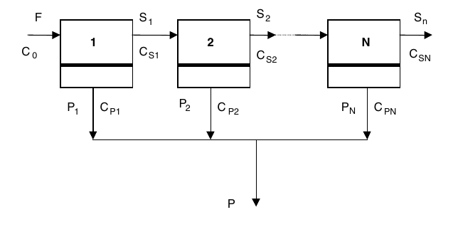
Ibarz, Fig. 10.13: single cascade layout, the layout Problem 10.2 works on (printed p. 299). The problem text cites Figure 10.2 for this layout.
Problem 10.3 is peach juice in two stages with recirculation: 18,000 kg/h at 11.5 Brix to 8950 kg/h at 23 Brix, at 50 C and 30 atm, with a membrane water permeability of 0.0117 mol/(s m2 atm). The book finds a final permeate of 9050 kg/h at 0.127 Brix, a first-stage permeate at 0.506 Brix, fluxes of 0.125 and 0.243 mol/(m2 s), areas of A_1 = 1149 m2 and A_2 = 574 m2, and a recirculation of 312 kg/h.
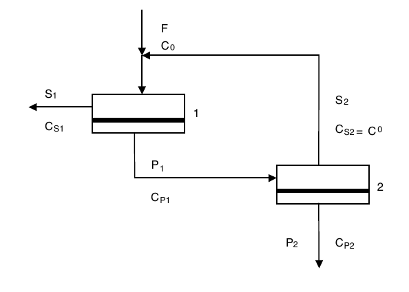
Ibarz, Fig. 10.14: two stage system with recirculation of the retained stream, the layout Problem 10.3 works on (printed p. 300).
Problem 10.4 is apple juice ultrafiltration: 12 Brix juice, a pectin gel at 4.5% w/V, feed pectin 0.5% w/V, a velocity of 1 m/s in tubes 1 cm in diameter and 2 m long, a density of 1020 kg/m3, a viscosity of 1.2 mPa.s, and a diffusivity of 8 x 10^-11 m2/s. The book finds Re = 8500, Sc = 1.47 x 10^4, Sh = 784, k_S = 6.27 x 10^-6 m/s, a flux of 1.38 x 10^-5 m3/m2 s, which is 49.62 l/m2 h, an area of 2.015 m2, and 32 tubes for 100 l/h.
Feed enters at the top left, the large particles stay above the membrane and leave as reject, and the small particles pass through the membrane and leave as permeate at the bottom right.
The basic membrane unit of Figure 10.2, shown again beside Problem 10.4: one stage, feed in, reject and permeate out.
Quick check
A whey ultrafiltration plant must pass 4595 kg/h of permeate at a flux of 30 kg/m2 h. How much membrane does it need?
Check your answer
153 m2: 4595 divided by 30, from Example 9.12.
10.9 What the books do and do not give
The membrane coverage in these books is Ibarz Chapter 10 plus the short Earle section, and this unit has used both. The outline for this subject says no worked example exists for membranes. That is corrected in section 10.7: Earle gives two worked examples, 9.11 and 9.12, and Ibarz gives four chapter problems with solutions. What the books do not give is a worked design example inside the Ibarz text itself: the design methods are procedures to follow, and the arithmetic sits in the chapter problems. The FPE papers listed in the outline for this unit, Wagner on ultrafiltration of milk, Kiviniemi on optimisation of an ultrafiltration process, and the papers on reverse osmosis of mandarin orange juice, milk and whey, and flux in laminar flow ultrafiltration, are supplementary conference papers, and no numbers from them are quoted here because the textbook chapters already carry the design material. One equation named in the outline, equation 10.69 for global recovery in two-stage recirculation, was not found on the page the outline cites, so it is not quoted here.
Try it yourself: Take a kitchen sieve, a piece of clean cotton cloth, and a coffee filter paper. Pour a glass of cloudy apple juice, or a glass of water with a spoonful of flour stirred in, through each one in turn. Note what passes and what stays, and how fast each one runs. The sieve stops only the largest bits, the cloth stops more, and the paper stops the most but runs the slowest. That is the membrane scale of section 10.1, and the slowing of the finest filter is the gel layer and the pore blocking of sections 10.4 and 10.6, in a kitchen.
Key ideas to carry forward
- A membrane splits a feed into a permeate that passes and a reject that stays, with no boiling and little energy.
- The four processes sit on one size scale: microfiltration stops suspension particles, ultrafiltration stops macromolecules, nanofiltration stops sugars, and reverse osmosis stops salts.
- Retention is R = 1 - C_P / C_C, and a molecular weight cut-off must be quoted with the percentage rejected below it.
- Water flows by osmosis from a dilute solution to a concentrated one, and reverse osmosis pushes it back with a pressure above the osmotic pressure, pi = i C R T.
- Osmotic pressure sets the plant pressure: coffee extract at 28% solids needs 3450 kPa, and apple juice at 15% solids needs 2070 kPa.
- Concentration polarization piles solute up at the membrane wall, raises the osmotic pressure there, and cuts the flux. Stirring thins the layer but never removes it.
- In reverse osmosis the solvent flux is J_D = A (Delta P - Delta pi) and the solute flux is J_S = B (C_C - C_P), so raising the pressure raises rejection toward 1 until compression and polarization limit it.
- In ultrafiltration a gel layer forms at the wall, and once it controls the flow the flux follows J = k_S ln(C_g / C_C) and stops rising with pressure.
- Earle gives two worked membrane examples, 9.11 and 9.12, correcting the outline note that said none exists. Example 9.11 gives a sucrose flow of 55 kg/m2 h at 10,000 kPa for a 10% solution, and Example 9.12 needs 153 m2 of membrane to concentrate whey protein twelve times.
- The book prints the sucrose molar concentration as 0.304 moles m-3, but the arithmetic uses the value as 0.304 kmol/m3, so the printed unit reads as a slip.
Glossary
Membrane
A thin barrier that lets some substances through and stops others. Food tech example: an ultrafiltration membrane that lets water, sugars and salts through but holds proteins back.
Permeate
The stream that passes through a membrane. Food tech example: the water leaving a reverse osmosis cell, or the watery stream leaving a whey ultrafiltration plant.
Reject
The stream held back by a membrane, also called the retentate or the concentrate. Food tech example: the protein-rich retentate left when whey is ultrafiltered.
Retentate
Another name for the reject: the stream that stays on the feed side of a membrane. Food tech example: the 8.6% protein retentate in Example 9.12.
Retention
The fraction of a substance held back by a membrane, R = 1 - C_P / C_C. Food tech example: a 95% retention of salt in Problem 10.1.
Molecular weight cut-off
The molecular weight above which a membrane retains most molecules, quoted with the percentage rejected below it. Food tech example: an ultrafiltration membrane with a cut-off chosen so a protein is retained and sugars pass.
Concentration factor
How much stronger the reject has become, F_C = C_S / C_F. Food tech example: whey protein concentrated by a factor of 12 in Example 9.12.
Recovery
How much of the feed is taken as permeate, Q = P / F. Food tech example: 89% recovery of salt water as permeate in Problem 10.1.
Osmosis
The movement of solvent through a semipermeable membrane from a dilute solution to a concentrated one. Food tech example: water moving into a strong sugar solution across a membrane.
Reverse osmosis
Applying a pressure above the osmotic pressure so the solvent flows from the concentrated side to the dilute side. Food tech example: taking water out of apple juice at 2070 kPa of osmotic pressure.
Osmotic pressure
The pressure that builds up when solvent moves by osmosis into a concentrated solution, given by pi = i C R T. Food tech example: 690 kPa for milk at 9% nonfat solids.
Concentration polarization
The piling up of solute at a membrane wall, raising the concentration there above the bulk liquid. Food tech example: the layer that slows an ultrafiltration membrane as protein gathers at its surface.
Gel layer
A layer of retained molecules at a membrane wall that behaves like a gel and adds its own resistance to flow. Food tech example: the pectin gel layer that limits the flux in apple juice ultrafiltration in Problem 10.4.
Flux
The flow through a membrane per unit of membrane area. Food tech example: a permeate flux of 30 kg/m2 h in whey ultrafiltration.
Module
The built unit that holds a membrane: flat, spiral or tubular in shape. Food tech example: a spiral module holding a large membrane area in a small volume.
References
- Ibarz, A., and Barbosa-Canovas, G. V., Unit Operations in Food Engineering, CRC Press, 2003. Chapter 10, Separation Processes by Membranes, including Figures 10.1, 10.2 and 10.3, Tables 10.1, 10.2 and 10.3, and Problems 10.1 to 10.4.
- Earle, R. L., Unit Operations in Food Processing, 2nd edition, Pergamon Press, 1983. Chapter 9, Contact-Equilibrium Separation Processes, membrane separations section, including Figure 9.9 and Examples 9.11 and 9.12.
- Cheryan, M., Ultrafiltration Handbook, as cited in Ibarz, Chapter 10, for Table 10.1.
- Lombardi, A. M., and Moresi, M., 1987, as cited in Ibarz, Chapter 10, for Table 10.2 and the design method.
- Perry, R. H., and Chilton, C. H., Chemical Engineer's Handbook, McGraw-Hill, New York, 1982, as cited in Ibarz, Chapter 10, for Table 10.3.
Unit 11: Mechanical Separations: Filtration, Centrifugation, Sedimentation and Fluidization
Note
Unit 11: Mechanical Separations: Filtration, Centrifugation, Sedimentation and Fluidization
Leave a glass of fresh milk on the bench and the cream rises to the top by itself. Spin the same milk fast enough and the cream comes off in seconds instead of hours. Pour a muddy liquid through a cloth and the cloth holds the mud while the liquid runs clear. Push air up through a bed of grain and the grain lifts, loosens and flows like a liquid. Four different machines, one idea: a force acts differently on things that differ in size or density, and the difference does the sorting. This unit follows that idea from a settling dust grain to a fluidized bed.
Questions to think about
- Why does a large particle settle faster than a small one, and by how much?
- How does a centrifuge turn a slow settling into a fast one, and what is the neutral zone in a cream separator?
- Why does a filter run slower as the cake grows, and what does washing the cake actually do?
- Why does a cyclone work well for coarse dust and poorly for fine dust?
- What happens when the air pushing up through a bed of particles pushes exactly as hard as gravity pulls down?
11.1 A particle in a fluid: how fast it settles
A particle in a fluid settles, or rises, at a terminal velocity where the driving force and the drag balance. For a sphere in streamline flow, Earle gives v_m = D^2 a (rho_p - rho_f) / (18 mu), equation 10.1, where D is the particle diameter, a is the acceleration, rho_p is the particle density, rho_f is the fluid density, and mu is the fluid viscosity. Under gravity, a = g, giving v_m = D^2 g (rho_p - rho_f) / (18 mu), equation 10.2. The drag coefficient in streamline flow is C = 24 / Re, and the streamline form holds for spheres with Re below 2.
Two things in that equation do most of the work. The velocity grows with the square of the diameter, so a particle twice as wide settles four times as fast. And it grows with the density difference, so a particle only slightly denser than the fluid settles slowly, while a much denser one falls fast. When the particle is less dense than the fluid, the sign flips and the particle rises: that is cream rising in milk, and oil globules rising in water.
Example 10.1: dust settling in air. A dust particle 60 micrometre in diameter, of density 1280 kg/m3, settles in air at 21 C, where the air viscosity is 1.8 x 10^-5 N s/m2 and the air density is 1.2 kg/m3. From equation 10.2 the settling velocity is 0.14 m/s. A particle of 10 micrometre settles at 3.9 x 10^-3 m/s. The Reynolds number for the larger particle is 0.56, so the flow is streamline and Stokes law applies. The small particle falls about 36 times more slowly than the large one, which is why fine dust hangs in the air of a mill long after the coarse dust has settled.
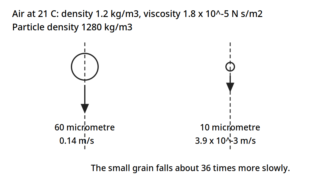
Two dust grains in air at 21 C. The 60 micrometre grain settles at 0.14 m/s and the 10 micrometre grain at 3.9 x 10^-3 m/s, so the fine dust hangs in the air long after the coarse dust has settled.
Diagram for Example 10.1: dust settling in air, drawn from the book data.
Quick check
Two particles of the same density settle in the same liquid. One is 20 micrometre across and the other is 10 micrometre across. How much faster does the larger one settle?
Check your answer
Four times as fast. Settling velocity grows with the square of the diameter, and 2 squared is 4.
11.2 Sedimentation: letting gravity do the work
At low concentration Stokes law applies, but in many practical cases the concentrations are too high. In concentrated suspensions, all particles appear to settle at a uniform velocity once a sufficiently high level of concentration is reached. Where the size range of the particles is not much greater than 10 to 1, all the particles tend to settle at the same rate. That is useful, because a thickener can then be designed on one settling velocity instead of a spread.
In a cylinder of uniform suspension allowed to settle, three zones appear: a zone of clear liquid at the top, a zone of more or less constant composition in the middle, settling at a uniform velocity, and a zone of sediment at the bottom. If the size range is wide, the constant-composition zone near the top will not occur and is replaced by an extended zone of variable composition. In a continuous thickener the same zones occur as the material flows through, with clarified liquid taken from the top and sludge from the bottom. The minimum area for a continuous thickener comes from equating the rate of sedimentation in a zone to the counter-flow velocity of the rising liquid: v_u = (F - L)(dw/d theta) / (A rho), where v_u is the upward velocity of the liquid, F is the mass ratio of liquid to solid in the feed, L is the mass ratio in the underflow, dw/d theta is the mass rate of feed of the solids, rho is the density of the liquid, and A is the settling area. If the settling velocity of the particles is v, then v_u = v, and A = (F - L)(dw/d theta) / (rho v), equation 10.3.
Example 10.2: a separating tank for oil and water. A continuous separating tank is to be designed to follow a water washing plant for a liquid oil. The oil, on leaving the washer, is in the form of globules 5.1 x 10^-5 m in diameter, the feed concentration is 4 kg of water to 1 kg of oil, and the leaving water is effectively oil free. The feed rate is 1000 kg/h, the density of the oil is 894 kg/m3, and the temperature of the oil and the water is 38 C. Assume Stokes law.
The viscosity of water is 0.7 x 10^-3 N s m-2, the density of water is 1000 kg/m3, and the diameter of the globules is 5.1 x 10^-5 m. From equation 10.2, v_m = (5.1 x 10^-5)^2 x 9.81 x (1000 - 894) / (18 x 0.7 x 10^-3) = 2.15 x 10^-4 m s-1 = 0.77 m h-1. Since F = 4 and L = 0, and dw/d theta, the flow of the minor component, is 1000 / 5 = 200 kg h-1, equation 10.3 gives A = 4 x 200 / (0.77 x 1000) = 1.0 m2. A tank of one square metre of settling area does the job, because the globules rise steadily and the water leaves clear.
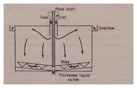
Earle, Fig. 10.1: continuous separating tank, the equipment Example 10.2 sizes (printed p. 146).
Equipment for gravitational sedimentation is built to give the settling time and to let the overflow and the sediment be removed without disturbing the separation. Continuous flow is generally desired, so the flow velocities are kept low, and vessels of various shapes are used, with slow-speed scraper-conveyors and pumps to remove the settled solids. When vertical cylindrical tanks are used, the scrapers generally rotate about an axis in the centre of the tank and the overflow is taken from the rim.
11.3 Cyclones, impingement and classifiers: sorting by inertia
A cyclone spins a gas stream so that centrifugal force throws the particles out of the stream. The force on a particle is F_c = m v^2 / r, equation 10.4, so for a fixed velocity the force rises as the radius falls: the smallest cyclones are the most efficient at removing small particles. The limits on smallness are the capital cost of small-diameter cyclones to provide sufficient output, and the pressure drops. Efficiency falls off for particles below about 10 micrometre in diameter, because the flow is complex and the size cut is not sharp.
Figure 11.1: Cyclone separator: (a) equipment, (b) efficiency of dust collection. (Earle, Fig. 10.2, p. 147.) The efficiency curve carries no numeric table in the book, so its path follows the printed shape; the axes, the tick labels 0 to 50 micrometre and 0 to 100%, and the proportions D, 2D and 2D are as the book gives them.
The efficient operation of a cyclone depends very much on a smooth double helical flow being produced. Anything that disturbs the flow or makes it depart from this pattern has a considerable adverse effect on efficiency: the air must enter tangentially at the top, and constricting baffles or lids should be avoided at the air outlet. Cyclones can be used for separating particles from liquids as well as from gases, and for separating liquid droplets from gases.
Impingement separators use the same idea in a different shape: deflector plates or rods, set normal to the direction of flow, abruptly change the direction of the gas, and the gas recovers its direction of motion more rapidly than the particles because of its lower inertia. Suitably placed collectors then catch the particles as they are thrown out of the stream. Mesh and fibrous air filters work on this principle. Where particle diameters fall below about 5 micrometre, cloth filters and packed tubular filters are about the only satisfactory equipment.
Classification means sorting particulate material into size ranges, using the different rates of movement of particles of different sizes and densities in a fluid, under gravity or centrifugal force. Rotary mechanical classifiers, combining differential settling with centrifugal action, have come into increasing use in flour milling: because of small differences in sizes, shapes and densities between starch and protein-rich material after crushing, the flour can be classified into protein-rich and starch-rich fractions. Classification is also used in direct air dryers, where the density decrease of material on drying is used to sort dry material out as a product and return wet material for further drying.
11.4 Centrifugation: gravity, multiplied
A centrifuge replaces gravity with centrifugal force. The force on a mass m at radius r turning with angular velocity omega is F_c = m r omega^2, equation 10.5, or F_c = m v^2 / r, equation 10.6. In the workshop form, F_c = 0.011 m r N^2, equation 10.7, with N in rev/min. The separation velocity becomes v_m = D^2 N^2 r (rho_p - rho_f) / (1640 mu), equation 10.8. The factor N^2 r is the whole point: double the speed and the force goes up four times, and a modest bowl at a few thousand rev/min gives hundreds of times gravity.
Example 10.3: how many g. A centrifuge turning at 2000 rev/min with a radius of 10 cm gives a force of 450 g. That single number explains why a centrifuge does in a minute what a settling tank does in an hour.
Earle, Fig. 10.3: liquid separation in a centrifuge, the machine of Example 10.3 (printed p. 148).
Example 10.4: oil in water, in a centrifuge. A dispersion of oil in water is to be separated using a centrifuge. The oil is dispersed as spherical globules 5.1 x 10^-6 m in diameter, of density 894 kg/m3. The centrifuge rotates at 1500 rev/min, the effective radius at which the separation occurs is 3.8 cm, the density of water is 1000 kg/m3, and its viscosity is 7 x 10^-4 N s/m2. This separation is the same as in Example 10.2, where the rate of settling under gravity was calculated.
From equation 10.8, v_m = (5.1 x 10^-6)^2 x (1500)^2 x 0.038 x (1000 - 894) / (1640 x 7 x 10^-4) = 0.02 m/s. Checking that Stokes law applies, Re = (5.1 x 10^-6 x 0.02 x 1000) / (7.0 x 10^-4) = 1.5, so the flow is streamline and it should obey Stokes law. Under gravity the same globules rose at 2.15 x 10^-4 m/s. In the centrifuge they move at 0.02 m/s, about 93 times as fast.
Earle, Fig. 10.4(a): centrifuge bowl geometry, the differential cylinder of Example 10.4 (printed p. 149).
In a liquid separator the two liquids must leave by different outlets, and the boundary between them sits at the neutral zone. For a vertical continuous liquid centrifuge, with the heavier liquid A discharging at radius r_1 and the lighter liquid B at radius r_2, the radius of the neutral zone is r_n^2 = (rho_A r_1^2 - rho_B r_2^2) / (rho_A - rho_B), equation 10.10. As the discharge radius for the heavier liquid is made smaller, the radius of the neutral zone must also decrease. In cream separation as much cream as possible is to be removed, so the neutral radius is kept small, and the feed should enter as nearly as possible into the neutral zone, so it enters with the least disturbance of the system.
Example 10.5: the neutral zone of a cream separator. A cream separator has discharge radii of 5 cm and 7.5 cm, the density of skim milk is 1032 kg/m3, and the density of cream is 865 kg/m3. Calculate the radius of the neutral zone so the feed inlet can be designed. From equation 10.10, r_n^2 = [1032 x (0.075)^2 - 865 x (0.05)^2] / (1032 - 865) = 0.022 m2, so r_n = 0.15 m. The feed should enter at 15 cm from the axis.
Earle, Fig. 10.4(b): the neutral zone, and Fig. 10.5: the disc-bowl centrifuges of Example 10.5 (printed pp. 149 to 150).
Brennan gives the same theory in the form of the equivalent settling area, Sigma: the flow a centrifuge can clarify is q = 2 v_g Sigma, where v_g is the settling velocity of the particle in a gravitational field and Sigma is characteristic of the centrifuge, equivalent to the area of a gravity settling tank with similar settling characteristics. For a simple cylindrical bowl, Sigma is approximately pi omega^2 b (3 R_2^2 + R_1^2) / (2 g), equation 7.20, and for a disc-bowl centrifuge, Sigma = 2 pi omega^2 (S - 1) (R_x^3 - R_y^3) / (3 g tan Omega), equation 7.21, where S is the number of discs in the stack and R_x and R_y are the outer and inner radius of the stack. Centrifuges of the same type but of different sizes have the same performance when q / Sigma is the same, which is the scale-up rule: keep q / Sigma constant.
The disc-bowl centrifuge is the workhorse of the dairy and the oil industry. Feed enters at the top, the discs rotate with the bowl, the dense phase travels toward the bowl wall and streams down the undersides of the discs, and the light phase, displaced toward the centre, flows over the upper faces of the discs. The liquids are thus divided into thin layers, the distance any drop must travel to be caught is very small, and the shearing at the liquid-liquid interface between the countercurrent streams can help to break up certain types of emulsion and improve separation. One note on the citation: the outline for this subject cites Brennan Fig. 7.5 at PDF page 155, but the page rendered at PDF 155 shows Fig. 7.7, the disc-bowl centrifuge. Fig. 7.5, the principle of the simple centrifugal filter, is on PDF page 152, printed page 136, and that is the page cited below.
Figure 11.2: Principle of simple centrifugal filter. (Brennan, Fig. 7.5, printed p. 136, PDF p. 152.)
The rate of flow of filtrate through a centrifugal filter, for an incompressible cake and neglecting kinetic energy changes, is given by Brennan equation 7.22, in which q is the volumetric flowrate of filtrate, rho is the filtrate density, omega is the rotational speed, R_1 is the radius of the inner surface of the liquid ring, R_2 is the radius of the inner surface of the cake, R_3 is the radius of the inner surface of the bowl, alpha is the specific cake resistance, M_c is the mass of solid cake in the basket, R_m is the resistance of the filter medium, and b is the height of the basket. Such an equation applies only to cakes of uniform thickness, and in most practical cases cakes are thicker near the base than the top, giving a filtration rate 5 to 20% greater than a cake of constant thickness of similar volume and permeability.
Brennan's equipment survey is worth keeping beside the theory. Tubular-bowl centrifuges are 3 to 6 inches in diameter and up to 5 ft high, with a typical unit 4 inches in diameter and 30 inches high running at 15,000 rev/min, and laboratory models up to 50,000 rev/min. Disc-bowl centrifuges run 8 to 40 inches in diameter, with disc spacing 0.02 to 0.05 inches, and a typical 12-inch bowl at 6,400 rev/min develops 7000 g. Desludging is provided when the solids content is greater than 5% or 6% by weight of feed. Batch filtering centrifugals have bowls 30 to 48 inches in diameter and 18 to 30 inches deep, running up to about 2000 rev/min, with a cycle of 3 to 30 minutes. The applications run through the food industry: tubular bowls for animal fats, vegetable and fish oils, fruit juices, cider and sugar syrup; disc-bowls for cream from milk, oil refining, fruit juices and citrus oils; conveyor-bowls for animal and vegetable protein, cocoa, coffee and tea slurries, fish oils and fish meal; filtering centrifugals for sugar refining, fruit and vegetable juice extraction, vegetable proteins and freeze concentration.
Quick check
A cream separator feed should enter at the neutral zone radius. In Example 10.5 that radius is 0.15 m. What goes wrong if the feed enters far from the neutral zone?
Check your answer
The feed disturbs the flow in the bowl, the two liquids mix again at the inlet, and the separation gets worse.
11.5 Filtration: a cake that grows and slows the flow
Filtration passes a liquid through a porous medium that holds the solids back. The solids build a cake on the medium, and the cake itself becomes the filter, so the flow slows as the cake grows. Earle gives the rate as dV/d theta = A Delta P / (mu r [w V/A + L]), equation 10.12, where V is the filtrate volume, A is the area, Delta P is the pressure drop, mu is the viscosity, r is the specific resistance of the cake, w is the mass of solids per unit volume of filtrate, and L is the equivalent thickness of the medium. At constant pressure this integrates to theta A / V = (mu r w / 2 Delta P)(V/A) + mu r L / Delta P, equation 10.14. A plot of theta A / V against V/A is a straight line, and its slope and intercept give the cake resistance and the medium resistance. Many cakes are compressible, so the resistance rises with pressure: r = r' (Delta P)^s, where s is 0 for an incompressible cake and rises toward 1.0 as compressibility increases.
Ibarz builds the same theory on the cake resistance alpha, in m/kg, and the medium resistance R_f, in m-1. The total rate is set by the pressure drop over the two resistances in series. At constant pressure, t/V = K_1 V + K_2, equation 9.27, with K_1 = eta / (2 A^2 (-Delta P) C), equation 9.25, and K_2 = R_f eta / (A (-Delta P)), equation 9.26. The flow is fastest at the start, q_max = A (-Delta P) / (eta R_f), equation 9.31, when the cake is thinnest. At constant flow, the pressure rises linearly with time, (-Delta P) = K_3 t + K_4, equation 9.36. Compressible cakes follow the Almy and Lewis form, alpha = alpha_0 (-Delta P_c)^n, equation 9.20, with n from 0.1 to 1, and the Ruth form, equation 9.21.
The plate-and-frame press filter is the classic batch filter. Plates and frames alternate in a stack, the feed enters at the bottom, passes through the filtering medium, and the filtrate leaves at the top. The cake builds in the frames, and when the frames are full the press is opened and the cakes are dropped out.
Figure 11.3: Filtration operation in a plate-and-frame press filter. (Ibarz, Fig. 9.3, p. 246.)
Cake washing is where filtration meets the washing of Unit 9. If the wash water follows the same path as the filtrate, it sweeps the soluble matter out fast: up to 90% of the solubles come out in the initial stage. If it follows a different path, the removal is gradual. In a plate-and-frame press the washing area is half the filtration area, the medium is crossed twice, and the washing flow is q_L = 1 / (8 K_1 V + 4 K_2), equation 9.39b, with the washing time t_L = V_L / q_L, equation 9.40.
A filter cycle is filtration plus washing plus the dead time of opening, emptying and closing: t_C = t + t_L + t*, equation 9.42. The capacity is F_c = V / t_CYCLE, equation 9.41. The optimum comes from the Sbarbaugh graphical method, and the book gives the result as t' = K_1 V^2, equation 9.44, with V_OPTIMUM = sqrt(t' / K_1), equation 9.45, and t_OPTIMUM = t' + K_2 sqrt(t' / K_1), equation 9.46.
The rotary vacuum filter runs the same filtration continuously. A drum covered with filter medium turns slowly in a trough of slurry. Vacuum inside the drum pulls filtrate through the medium while the drum is submerged, a cake builds on the outside, wash water sprays on the cake as it rises out of the trough, air dries it, and a scraper peels it off before the drum dips back in. The submerged time for a section is t_S = phi / (2 pi N), equation 9.47, where phi is the immersion angle and N is the rotation velocity.
Figure 11.4: Rotary vacuum filter. (Ibarz, Fig. 9.6, p. 251.) The spokes and the drum follow the book's arrangement, and all labels are as the book gives them.
Example 10.6: from a laboratory test to a plant filter. A filtration test was carried out on a laboratory filter press at 340 kPa, with an area of 0.186 m2. The filtrate collected was 20, 40, 60 and 80 kg at 8, 26, 54.5 and 93 minutes. Plotted as theta A / V against V/A, the graph gives a slope of 0.0265 and an intercept of 1.6, so theta / (V/A) = 0.0265 (V/A) + 1.6. For a plant filter at 270 kPa, with a concentration 50% greater, the same form gives theta / (V/A) = 0.0265 (340 / 270) (150 / 100) (V/A) + 1.6 (340 / 270) (150 / 100) (V/A). The plant filter area is 9.3 m2, and at V/A = 250 kg/m2 the total filtrate is 250 x 9.3 = 2325 kg in 1 hour. One small press, four timed weighings, and the size of the plant filter follows.
Other filter forms in the books are the rotary vacuum drum, the centrifugal filter of section 11.4, and air bag filters. Filter aids, including kieselguhr, are added to the feed or precoated on the medium to keep the cake open and the flow up. Brennan lists the applications: sugar cane and beet, starch, gluten, edible oils and their winterisation, breweries, and the clarification of beer, wines, vinegar, fruit juices, yeast and meat extracts, oils, brines, syrups and jellies, and the removal of micro-organisms.
11.6 Sieving: sorting by size alone
Sieving sorts dry particles by size, passing them through a mesh and keeping what is too big. The Tyler series uses a ratio of the square root of 2 between successive sieves, and standard sieves run from 25 mm down to about 0.6 mm, with industrial screening from 50 micrometre upwards. The result is a size distribution: how much of the powder sits between each pair of sieves.
Example 10.7: a powder in fractions. A powder is sieved, and 13% of it sits between 0.300 and 0.350 mm, and 9% sits between 0.350 and 0.400 mm. Those two numbers are the kind of result a sieve analysis gives: not one size, but the share of the powder in each size band. A miller reads that distribution to judge whether the grinding is right, and a food maker reads it to judge whether a powder will flow, dissolve and mix as it should.
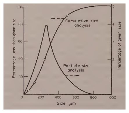
Earle, Fig. 10.9: particle-size analysis, the cumulative and distribution curves Example 10.7 reads (printed p. 156).
11.7 Fluidization: when a bed of solids flows like a liquid
Push a fluid up through a bed of particles and the pressure drop rises with the flow. At first the bed stays fixed. Then the drag on the particles equals their weight, the bed loosens, and the particles hang suspended in the stream: the bed is fluidized. Push harder still and the particles are carried away, which is pneumatic transport. Ibarz draws this as a curve with segments: OA, the fixed bed; AB, the rise to fluidization; BC, the fluidized bed at a steady pressure drop; and D, the transport region. The fluid velocity at the point of fluidization is the minimum fluidization velocity, v_mf, and the velocity at which particles are carried out is the drag velocity, v_D.
Flow through a fixed bed follows Darcy's law, v = K (-Delta P) / L, equation 8.1, or v = (1 / (alpha eta L)) Delta P, equation 8.2, where K is the permeability and alpha is the resistance. The Darcy unit is defined as 1 ml/(s.cm2) of a 1 cP liquid under 1 atm/cm. The bed is described by its specific surface and its porosity, with a_S = a_S0 (1 - epsilon), equation 8.3, where a_S0 is the specific surface of the particles and epsilon is the void fraction, and the equivalent diameter d_P = Gamma d_r, where Gamma is the sphericity factor. For a sphere Gamma is 1, and for other shapes it is lower, as Table 11.1 shows.
The pressure drop through the bed follows the Kozeny-Carman equation for laminar flow, equation 8.8, with K'' = 5 plus or minus 0.5, or 4.8 plus or minus 0.3 for spheres, the Burke-Plummer equation for turbulent flow, equation 8.10, and the Ergun equation for both, equation 8.13: (-Delta P) / L = 150 (1 - epsilon) eta v / (epsilon^3 d_P^2) + 1.75 (1 - epsilon) rho v^2 / (epsilon^3 d_P). The flow is laminar for Re_p below 40 and turbulent above 40. The Chilton-Colburn equation, equation 8.14, gives the mass transfer in the bed.
At the minimum fluidization velocity the drag balances the weight of the bed, equation 8.17, giving v_mf for laminar flow, equation 8.18, for turbulent flow, equation 8.19, and for the transition, equation 8.20. The minimum porosity is epsilon_mf = 1 - 0.356 log(d_P - 1), equation 8.21, with d_P in microns, valid from 50 to 500 micrometre. As the bed expands, the height follows L_1 (1 - epsilon_1) = L_2 (1 - epsilon_2), equation 8.22, because the mass of solids stays the same while the voids grow.
Table 11.1: Sphericity of particles (Ibarz Table 8.1, from Levenspiel, 1993)
| Form of the particle | Sphericity |
|---|---|
| Sphere | 1 |
| Cube | 0.81 |
| Cylinders, h = d | 0.87 |
| Cylinders, h = 5d | 0.70 |
| Cylinders, h = 10d | 0.58 |
| Discs, h = d/3 | 0.76 |
| Discs, h = d/6 | 0.60 |
| Discs, h = d/10 | 0.47 |
| Beach sand | As high as 0.86 |
| River sand | As low as 0.53 |
| Other types of sand | 0.75 |
| Triturated solids | 0.5-0.7 |
| Granulated particles | 0.7-0.8 |
| Wheat | 0.85 |
| Raschig rings | 0.26-0.53 |
| Berl chairs | 0.30-0.37 |
Table 11.1: Sphericity of particles. (Ibarz, Table 8.1, p. 225.)
The Ibarz chapter problems carry the fluidization arithmetic. Problem 8.1, cubic particles of 5 mm side, gives an equivalent diameter of 4.05 mm, a porosity of 0.512, a pressure loss of 2047 Pa/m, and Re_p = 203, which is turbulent. Problem 8.2 gives a pressure drop of 36,762 Pa over 3 m with Re_p = 153. Problem 8.3, peas with air at 5000 m3/h, gives a pressure drop of 50,979 Pa/m, which is 0.52 atm, with Re_p = 795. Problem 8.4, hollow glass rings, gives a mass flux of 2.074 kg/(m2 s), a mass flow of 1.629 x 10^-2 kg/s, a volumetric flow of 16.3 l/s, and Re_p = 988.
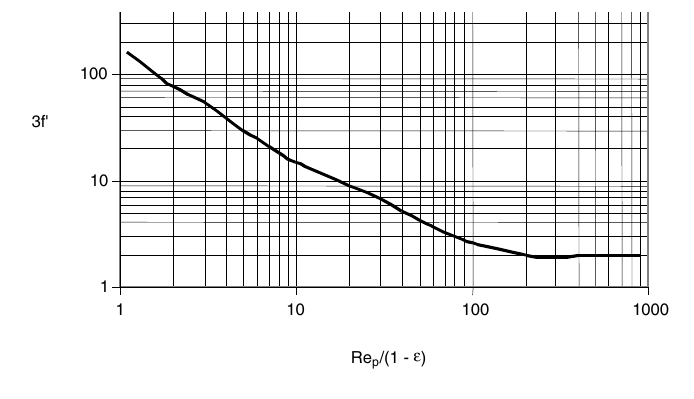
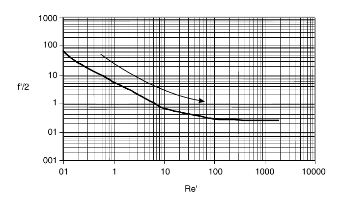
Ibarz, Fig. 8.1 and Fig. 8.2: the friction-factor plots the pressure drop in Problems 8.1 to 8.4 is read from (printed pp. 214 to 215).
Problem 8.5, cylindrical particles, gives a specific surface of 1777.74 m-1, a porosity of 0.6, and a bed specific surface of 711.1 m-1.
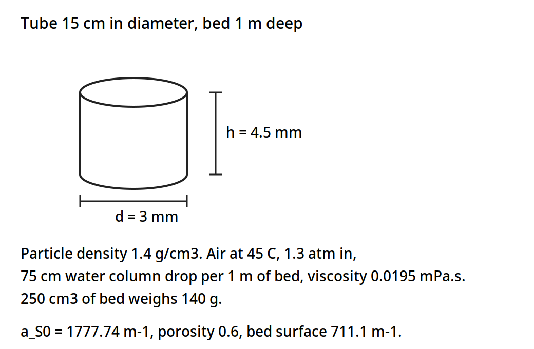
A cylindrical particle 3 mm across and 4.5 mm high, in a 15 cm tube. The book gives a particle specific surface of 1777.74 m-1, a porosity of 0.6 and a bed specific surface of 711.1 m-1.
Diagram for Ibarz Problem 8.5: cylindrical particles, drawn from the book data.
The filtration problems, 9.1 to 9.5, give capacities from 3.91 l/min to 87.42 l/min, cake resistances from 6.07 x 10^9 to 2.75 x 10^10 m/kg, and a rotary drum area of 11.73 m2 with a cake thickness of 18 mm in Problem 9.5.
The book gives each filtration problem its own numbers. Problem 9.1: a plate-and-frame filter under constant pressure needs 1 h to separate 600 l of filtrate of an aqueous suspension, the initial filtration velocity is 60 l/min, 8 l of water are needed to wash the deposited cake, and 35 min are needed to discharge, clean and assemble the filter. Problem 9.2: a plate-and-frame press filter works under constant filtration velocity, 250 l of filtrate are obtained after 45 min, and during this period the pressure drop increases from 0.40 kg/cm2 to 3.5 kg/cm2; the question is what amount of filtrate would be obtained after 45 min at a constant pressure of 3.5 kg/cm2. Problem 9.3: an aqueous suspension that contains 7% of insoluble solids is filtered at a rate of 10 ton/h, using a plate-and-frame press filter under a constant pressure of 3 atm; the deposited cake contains 50% moisture, the density of the dry solids is 3.5 g/cm3, and the equivalent diameter of the deposited particles is 0.002 mm; washing begins after 10,000 kg/h of feeding have been filtered using 150 l of water, while 30 min are used for discharge, cleaning and assembly, and the resistance of the filtering medium is negligible. Problem 9.4: an aqueous solution that contains 10% suspended solids is filtered in a plate-and-frame press filter; the wet cake to dry cake ratio is 2.2, using an incompressible cake with a specific resistance of 2.5 x 10^10 m/kg; filtration runs at a constant pressure of 3 atm, and the filtrate masses recorded are 1600 kg at 8 min, 2700 kg at 18 min, 3720 kg at 31 min, 4900 kg at 49 min, 6000 kg at 70 min and 7125 kg at 95 min. Problem 9.5: 60 l/min of filtrate are wanted from an aqueous suspension that contains 0.25 kg of insoluble solids per kg of water, using a rotary drum filter; the pressure drop is 300 mm of Hg, the cake has 50% moisture, the filtrate has a viscosity of 1.2 mPa.s and a density of 1000 kg/m3, the filter cycle time is 5 min with 30% of the total surface submerged, and the particles are spheres of 6 x 10^-3 mm diameter and 900 kg/m3 density, with the medium resistance negligible and a Kozeny constant of 5.
Figure 11.3, shown again beside Problems 9.1 to 9.4: the plate-and-frame press filter those four problems work on.
Figure 11.4, shown again beside Problem 9.5: the rotary vacuum filter that problem sizes.
Quick check
Air is blown up through a bed of peas, and the pressure drop stops rising as the flow rises. What has happened to the bed?
Check your answer
The bed has fluidized. The drag now balances the weight of the particles, so the pressure drop stays steady while the bed expands.
11.8 What the books do and do not give
Earle gives the worked examples in this unit, 10.1 to 10.7, with the numbers checked twice against the page images. Ibarz gives the theory of porous beds and filtration, with end-of-chapter problems and solutions, and no worked examples inside the text. Brennan gives the centrifuge theory, the Sigma method, and the equipment survey, with the figure citation corrected in section 11.4: Fig. 7.5 is on PDF page 152, printed page 136, not PDF page 155 as the outline says. The outline's Fig. 7.5 citation is the one figure page in this unit that did not match the book, and it is corrected here rather than repeated.
Try it yourself: Stir a spoonful of flour into a tall glass of water and watch it settle. Time how long the cloud takes to clear, then stir in a spoonful of coarse sugar and compare. The sugar clears first, because its particles are larger and denser. Then pour the flour water through a coffee filter and watch the flow slow as the cake builds: that is the filtration of section 11.5, with the flow falling as the cake grows. Wash the cake with a little clean water and see the wash run clearer than the first filtrate.
Key ideas to carry forward
- A particle settles at v_m = D^2 g (rho_p - rho_f) / (18 mu), so doubling the diameter makes it settle four times as fast.
- In concentrated suspensions the particles settle at a uniform velocity, and a thickener is sized on that velocity: the oil-water tank of Example 10.2 needs 1.0 m2.
- A cyclone throws particles out by centrifugal force, F_c = m v^2 / r, and its efficiency falls off below about 10 micrometre.
- A centrifuge multiplies gravity: 2000 rev/min at 10 cm gives 450 g, and the oil globules of Example 10.4 move at 0.02 m/s instead of 2.15 x 10^-4 m/s under gravity.
- The neutral zone of a cream separator sits at r_n = 0.15 m for discharge radii of 5 cm and 7.5 cm, and the feed should enter there.
- A filter slows as its cake grows, and the constant-pressure plot of theta A / V against V/A is a straight line whose slope and intercept give the cake and medium resistances.
- A laboratory test at 340 kPa sizes a plant filter of 9.3 m2 that collects 2325 kg of filtrate in 1 hour, in Example 10.6.
- The rotary vacuum filter runs filtration continuously: vacuum while submerged, wash water, air drying, and a scraper.
- A fluidized bed hangs its particles in the gas stream when the drag balances their weight, and the Ergun equation gives the pressure drop through the bed.
- Sphericity runs from 1 for a sphere to 0.26 for a Raschig ring, and wheat sits at 0.85.
- Brennan Fig. 7.5 is on PDF page 152, printed page 136, not PDF page 155 as the outline says.
Glossary
Terminal velocity
The steady speed a particle reaches when the driving force and the drag on it balance. Food tech example: a 60 micrometre dust grain settling in air at 0.14 m/s.
Stokes law
The law for the settling velocity of a sphere in streamline flow, v_m = D^2 g (rho_p - rho_f) / (18 mu). Food tech example: oil globules rising in water in Example 10.2.
Sedimentation
Separation by letting particles settle, or droplets rise, under gravity. Food tech example: cream rising in milk, or oil globules rising from wash water in a separating tank.
Thickener
A vessel in which a suspension settles continuously, with clear liquid overflowing at the top and thickened sludge leaving at the bottom. Food tech example: the continuous separating tank of Example 10.2.
Cyclone
A separator that spins a gas stream so centrifugal force throws the particles to the wall. Food tech example: a cyclone taking flour dust out of mill air.
Centrifuge
A machine that spins a bowl fast so centrifugal force separates liquids or solids far faster than gravity. Food tech example: a cream separator running at thousands of rev/min.
Neutral zone
The surface inside a liquid centrifuge where the two liquids meet, set by the discharge radii and the densities. Food tech example: the 0.15 m neutral radius in a cream separator.
Sigma
The equivalent settling area of a centrifuge: the area of a gravity settling tank that would do the same work. Food tech example: scaling a centrifuge up by keeping q / Sigma constant.
Disc-bowl centrifuge
A centrifuge whose bowl holds a stack of closely spaced conical discs that split the liquids into thin layers. Food tech example: the standard machine for taking cream from milk.
Filtration
Passing a liquid through a porous medium that holds the solids back. Food tech example: clarifying fruit juice on a plate-and-frame press filter.
Cake
The layer of solids that builds on a filter medium and itself becomes the filter. Food tech example: the cake in the frames of a plate-and-frame press.
Specific cake resistance
A measure of how hard it is to push liquid through a cake, in m/kg. Food tech example: a cake resistance of 6.07 x 10^9 m/kg in Ibarz Problem 9.3.
Filter aid
A porous material added to a feed or precoated on a medium to keep the cake open and the flow up. Food tech example: kieselguhr used in clarifying beer.
Rotary vacuum filter
A drum filter that turns in a trough of slurry, filtering under vacuum while submerged and discharging the cake by a scraper. Food tech example: the drum filter of Figure 11.4.
Sieving
Sorting dry particles by passing them through meshes of known opening. Food tech example: a Tyler sieve series separating a ground spice into size fractions.
Fluidization
Hanging solid particles in an upward stream of fluid so the bed loosens and flows like a liquid. Food tech example: air fluidizing a bed of peas for drying.
Minimum fluidization velocity
The upward fluid velocity at which the drag on the particles just balances their weight and the bed loosens. Food tech example: the velocity v_mf at the top of the fixed-bed curve.
Porosity
The fraction of a bed that is empty space between the particles. Food tech example: a bed porosity of 0.512 for cubic particles in Ibarz Problem 8.1.
Sphericity
A factor from 0 to 1 that says how close a particle is to a sphere, used to find its equivalent diameter. Food tech example: wheat at 0.85, a cube at 0.81, a sphere at 1.
References
- Earle, R. L., Unit Operations in Food Processing, 2nd edition, Pergamon Press, 1983. Chapter 10, Mechanical Separations, including Figure 10.2 and Examples 10.1 to 10.7.
- Ibarz, A., and Barbosa-Canovas, G. V., Unit Operations in Food Engineering, CRC Press, 2003. Chapter 8, Circulation of Fluid through Porous Beds: Fluidization, including Table 8.1 and Problems 8.1 to 8.5; Chapter 9, Filtration, including Figures 9.3 and 9.6 and Problems 9.1 to 9.5.
- Brennan, J. G., Butters, J. R., Cowell, N. D., and Lilly, A. E. V., Food Engineering Operations, Elsevier, 1969. Chapter 6, Filtration and Expression; Chapter 7, Centrifugation, including Figure 7.5 and the Sigma method.
- Levenspiel, O., Flujo de Fluidos: Intercambio de Calor, Reverti, Barcelona, 1993, as cited in Ibarz, Chapter 8, for Table 8.1.
Unit 12: Size Reduction, Mixing and Emulsification
Note
Unit 12: Size Reduction, Mixing and Emulsification
A wheat kernel becomes flour, a spice berry becomes a powder that colours a whole pot, and a spoonful of oil and a spoonful of water that would never mix become mayonnaise that holds together for weeks. Three different moves, one thread: the size of the pieces and the evenness of the mixture decide how a food behaves, how it flows, how it dissolves, and how long it keeps. How much power does it take to make things smaller, how do you know when a mixture is mixed enough, and how do you keep two liquids that hate each other together? This unit follows those three questions from the mill to the mixer to the homogenizer.
Questions to think about
- Why does grinding a powder finer take so much more power than grinding it coarse?
- How can a maker tell, with numbers, whether a powder mixture is well mixed or still patchy?
- Why does a tiny pinch of vitamin powder need five stages of mixing to reach a tonne of cereal evenly?
- Why does a mixing tank need baffles, and what goes wrong when a vortex forms?
- How does a homogenizer break fat into droplets so small that cream stops rising in milk?
- What turns cream into butter, and why is that the same science as making mayonnaise, in reverse?
12.1 Why make things smaller
Size reduction has four reasons in a food plant. It makes a material easier to handle and to pack. It opens up surface so that later steps, such as extraction, drying and cooking, work faster. It makes a mixture more even, because small pieces blend better than large ones. And it makes a product of the size the customer wants, from a coarse cracker crumb to a fine flour.
The forces are three: compression, as in crushing rolls and jaw crushers; impact, as in hammer mills; and shear, as in disc attrition mills. Brennan's table of forces puts crushing rolls under compression, hammer mills under impact, and disc attrition mills under shear. The reduction ratio is the average size of the feed over the average size of the product: coarse crushers work below 8 to 1, and fine grinding reaches up to 100 to 1. Hardness, fibrous structure and moisture all shape the choice. Moisture above 2% to 3% causes clogging and balling in a mill. Dust brings two hazards: inhalation and explosion, because a fine powder in air can burn fast. Grinding also makes heat, and heat can damage flavour and nutrients, so mills are often cooled or run in short passes.
Gould's plant chapters add the gentler end of the same work. Disintegration with little change in form is husking, pitting, coring, shelling and snipping: the food keeps its shape and loses only a part. Disintegration with considerable change in form is cutting, shredding, crushing, comminuting, homogenizing and juicing: the food is broken down into a new form. The two chapters sit at the front of the factory, where the raw material is prepared for the operations this unit describes.
Quick check
A mill feed is wet, above 3% moisture, and the mill keeps clogging. Is the answer more power, or drier feed?
Check your answer
Drier feed. Moisture above 2% to 3% causes clogging and balling, and more power only makes more heat and more paste.
12.2 How much power: Kick, Rittinger and Bond
The energy of grinding follows a general form, dE/dL = K L^n, equation 11.1, where dE is the differential energy required, dL is the change in a typical dimension, L is the magnitude of that dimension, and K and n are constants. Three laws come from three values of n.
Kick assumed the energy was directly proportional to the size reduction ratio, dL/L, so n is -1, and the energy is E = K_K f_c log_e(L_1 / L_2), equation 11.2, where K_K is Kick's constant and f_c is the crushing strength of the material. The same specific energy crushes a material from 10 cm to 5 cm as from 5 mm to 2.5 mm. Kick's law fits coarse grinding, where the increase in surface area per unit mass is relatively small.
Rittinger assumed the energy was directly proportional to the change in surface area, not to the change in length, so n is -2, and E = K_R f_c (1/L_2 - 1/L_1), equation 11.3, where K_R is Rittinger's constant. The same energy that reduces particles from 10 cm to 5 cm would reduce the same mass of 5 mm particles down to 4.7 mm: a very much smaller reduction, because the smaller particles already carry so much surface. Rittinger's law fits fine powders, where large areas of new surface are being created.
Bond suggested an intermediate course, with n = -3/2, giving E = E_i (100/L_2)^(1/2) (1 - 1/q^(1/2)), equation 11.4, where q = L_1/L_2 is the reduction ratio, L is in microns, and E_i is the work index: the energy required to reduce unit mass from an infinitely large particle size down to a particle size of 100 micrometre. All three equations are dimensional equations, so the quoted values must be used with the dimensions expressed in appropriate units: in Bond's equation, if L is expressed in microns, the equation defines E_i. Less than 2% of the input energy appears as increased surface energy: the rest becomes heat, noise and motion, which is why grinding is expensive and hot.
Example 11.1: sugar, and the motor that was just enough. Sugar is ground from crystals of which 80% pass a 500 micrometre sieve, down to a size in which 80% passes an 88 micrometre sieve, and a 5 horsepower motor is found just sufficient for the required throughput. If the requirements are changed so that the grinding is only down to 80% through a 125 micrometre sieve, but the throughput is to be increased by 50%, would the existing motor have sufficient power to operate the grinder? Assume Bond's equation.
Using the subscripts 1 for the first condition and 2 for the second, and letting W kg/h be the initial throughput, with x the required power: E_1 = 5/W = E_i (100 / 88 x 10^-6)^(1/2) [1 - (88/500)^(1/2)], and E_2 = x / 1.5W = E_i (100 / 125 x 10^-6)^(1/2) [1 - (125/500)^(1/2)]. Dividing, E_2/E_1 = x / (1.5 x 5) = (88 x 10^-6)^(1/2) [1 - (125/500)^(1/2)] / (125 x 10^-6)^(1/2) [1 - (88/500)^(1/2)]. So x / 7.5 = 0.84 x 0.500 / 0.58 = 0.72, and x = 5.4 horsepower. The motor would have insufficient power to pass the 50% increased throughput, though it should be able to handle an increase of 40%. A coarser grind does not save enough power to pay for half as much more material.
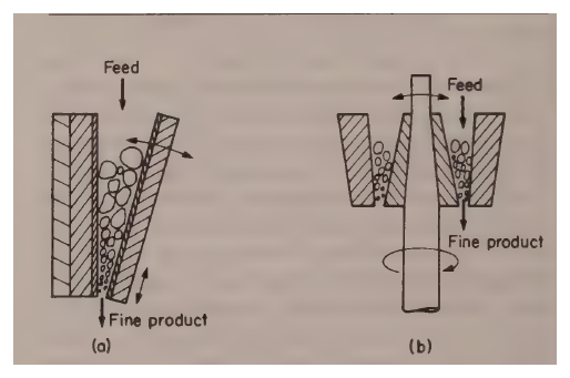
Figure 12.1, shown again beside Example 11.1: the jaw and gyratory crushers that grind the sugar.
12.3 The new surface: why fine powders behave differently
When a uniform particle is crushed, the sizes produced vary a great deal at first, from relatively coarse to fine dust. As grinding goes on, the coarser particles are further reduced while the fine ones change less, and a certain size tends to increase in its relative proportions and soon becomes the predominant size fraction. Wheat after first crushing gives a wide range of particle sizes in the coarse flour, but after further grinding the predominant fraction soon becomes that passing a 250 micrometre sieve and being retained on a 125 micrometre sieve, and this fraction tends to build up however long the grinding continues, so long as the same type of machinery is used.
The surface area of a fine powder is large and it matters. Most reactions are related to the surface area available, so the surface area can have a considerable bearing on the properties of the material. Wheat in the form of grains is relatively stable so long as it is kept dry, but ground to a fine flour it has such a large surface per unit mass that it becomes liable to explosive oxidation, as is all too well known in the milling industry.
The surface area to volume ratio of a particle is A_s/V_s = 6 lambda / D_s, equation 11.5, where lambda is a shape factor, about 1.75 for ground materials and 1 for a cube or a sphere. The total area of a mass w of particles of density rho_p is A_s = 6 lambda w / (rho_p D_s), equation 11.6. Combined with the results of a sieve analysis, that equation estimates the total surface area of a powder.
Example 11.2: the surface area of ground salt. In an analysis of ground salt using Tyler sieves, it was found that 38% of the total salt passed through a 7-mesh sieve but was caught on a 9-mesh sieve. For one of the finer fractions, 5% passed an 80-mesh sieve but was retained on a 115-mesh sieve. Estimate the surface areas of these two fractions in a 5 kg sample of the salt, if the density of salt is 1050 kg/m3 and the shape factor is 1.75.
The aperture of Tyler sieves is 7 mesh = 2.83 mm, 9 mesh = 2.00 mm, 80 mesh = 0.177 mm, and 115 mesh = 0.125 mm. The mean aperture of 7 and 9 mesh is 2.41 mm, and the mean aperture of 80 and 115 mesh is 0.151 mm. So A_1 = (6 x 1.75 x 0.38 x 5) / (1050 x 2.41 x 10^-3) = 7.88 m2, and A_2 = (6 x 1.75 x 0.05 x 5) / (1050 x 1.51 x 10^-4) = 16.6 m2. The fine fraction is only 5% of the mass but carries more than twice the surface of the coarse fraction that holds 38% of the mass. That is why a little fine dust changes a powder so much: it brings the surface with it.
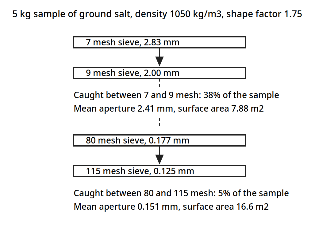
Two fractions of the same 5 kg of ground salt. The coarse fraction holds 38% of the mass and carries 7.88 m2 of surface; the fine fraction holds only 5% of the mass and carries 16.6 m2.
Diagram for Example 11.2: sieve stack for ground salt, drawn from the book data.
Quick check
A powder has 5% of its mass in a fine fraction and 38% in a coarse fraction. Which fraction carries more surface area, and why?
Check your answer
The fine fraction: 16.6 m2 against 7.88 m2 in Example 11.2, because surface area per unit mass grows as the particle size falls.
12.4 Grinding equipment: crushers, mills and screens
Grinding equipment divides into two classes: crushers, where the major action is compressive, and grinders, which combine shear and impact with compressive forces. Jaw and gyratory crushers are heavy equipment and are not used extensively in the food industry, but they show the principle clearly. In a jaw crusher the material is fed between two heavy jaws, one fixed and the other reciprocating, working the material down into a narrower space and crushing it as it goes. The gyratory crusher is a truncated conical casing inside which a crushing head rotates eccentrically: the head is shaped as an inverted cone, and the material is trapped between the outer fixed cone and the inner gyrating cone and forced into a narrower space, where it is crushed.
Figure 12.1: Crushers: (a) jaw, (b) gyratory. (Earle, Fig. 11.1, p. 162.)
Crushing rolls are two heavy cylinders mounted parallel and close together, rotating in the same direction, trapping the material in the nip and crushing it as it passes through. They may be driven at the same speed or at differential speeds, and a major application is in the cane-sugar industry, where several stages of rolls crush the cane. The angle of nip follows cos(A/2) = (D_r + D_p) / (D_r + D_f), where D_r is the roll diameter, D_p is the nip opening, and D_f is the feed size, and the limiting case is tan(A/2) = mu, where mu is the coefficient of friction. The theoretical capacity is Q = 60 pi N D_r D_p l ft3/hr, for a roll diameter D_r in feet, a length of face l in feet, and a speed N in rev/min, and the actual capacity is 0.1 to 0.3 of the theoretical. Rolls run at 50 to 300 rev/min, and the reduction ratio is usually below 5.
The hammer mill is the common fine grinder of the food industry. Swinging hammer heads are attached to a rotor turning at high speed inside a hardened casing, and the material is crushed and pulverized between the hammers and the casing, remaining in the mill until it is fine enough to pass through a screen forming the bottom of the casing. Both brittle and fibrous materials can be handled in hammer mills, though with fibrous material, projecting sections on the casing may be used to give a cutting action.
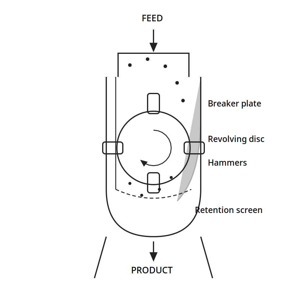
Feed drops onto the revolving disc, the hammers throw the pieces against the breaker plate and the casing, and only particles fine enough to pass the retention screen leave as product.
Figure 12.2: A hammer mill. (Brennan, Fig. 4.3, p. 51.)
Other mills in the books are the disc attrition mill, single and double, the Buhr mill, and the ball mill, in which the material is ground by tumbling balls inside a rotating cylinder. The critical speed of a ball mill is N_c = 76.6 / sqrt(2R) rev/min, with R in feet, and the optimum speed is about 75% of the critical: too slow and the balls slide, too fast and they centrifuge to the wall and stop grinding. Mills run in open circuit, in free crushing, in choke feeding, or in closed circuit with a screen returning the oversize. Wet milling is used where a slurry suits the later steps.
Screening sorts the product after grinding. The undersize that passes is the fines or minus, the oversize that stays is the tails or plus. The mesh number counts the openings per inch, and the Tyler ratio of the square root of 2 sets the steps of the series. A trommel, a rotating cylindrical screen, has the same critical speed formula as a ball mill. Screening efficiency turns on the feed rate, the particle size and alignment, the moisture, worn screens, and blinding, where near-size particles plug the openings.
12.5 Rheology: how the food flows decides how it mixes
Mixing is governed by how the material flows, and Ibarz Chapter 6 gives the rheology that a mixer designer needs. A Newtonian liquid has a viscosity that does not change with the rate of shear: water, milk, filtered juices and honey behave this way over the usual range. A non-Newtonian liquid changes its apparent viscosity as it is sheared. Most foods are non-Newtonian: ketchup and mustard flow more easily the harder they are pushed, which is pseudoplastic flow, and some pastes need a push to start flowing at all, which is a yield stress.
The power law describes the common case, with a consistency coefficient m and a flow index n. When n is below 1, the fluid is pseudoplastic; when n is 1, it is Newtonian; and the Bird-Leider model extends the power law to long times, converging to the power law and describing the shear stress overshoot peaks. Some semiliquid products are viscoelastic, showing the properties of a viscous liquid and an elastic solid together: a Newtonian liquid squirted through a pipe contracts as it leaves, while a viscoelastic fluid widens markedly, the Barus effect, and a viscoelastic fluid stirred with a small rod climbs up the rod, the Weissenberg effect, instead of forming a vortex that dips down.
Table 12.1 shows how fast viscosity rises with sugar concentration: a sucrose solution at 20% holds a viscosity of 2.0 mPa.s at 20 C, and at 75% it holds 2344.0 mPa.s. That thousandfold rise is why a syrup and a juice need different mixers, different speeds and different power.
Table 12.1: Viscosity coefficients of sucrose solutions at 20 C (Ibarz Table 6.1, from Muller, 1973)
| Sucrose % | g/100 g water | Viscosity (mPa.s) |
|---|---|---|
| 20 | 25.0 | 2.0 |
| 25 | 33.2 | 2.5 |
| 30 | 42.9 | 3.2 |
| 35 | 53.8 | 4.4 |
| 40 | 66.7 | 6.2 |
| 45 | 81.8 | 9.5 |
| 50 | 100.0 | 15.5 |
| 55 | 122.2 | 28.3 |
| 60 | 150.0 | 58.9 |
| 65 | 185.7 | 148.2 |
| 70 | 233.3 | 485.0 |
| 75 | 300.0 | 2344.0 |
Table 12.1: Viscosity coefficients of sucrose solutions at 20 C. (Ibarz, Table 6.1, p. 117.)
Table 12.2 gives the power law and Bird-Leider parameters for fifteen foods, from Kokini (1992). Honey is nearly Newtonian, with n = 0.989. Ketchup, mayonnaise, mustard and peanut butter are strongly pseudoplastic, with n from 0.065 to 0.196, so they flow far more easily once they are moving. Peanut butter carries the largest consistency coefficient in the table, m = 501.13 Pa.s^n, and the longest relaxation time, lambda = 1.86 x 10^5 s.
Table 12.2: Rheological parameters of foods (Ibarz Table 6.3, from Kokini, 1992)
| Food | m (Pa.s^n) | n | m' (Pa.s^n') | n' | lambda (s) |
|---|---|---|---|---|---|
| Apple marmalade | 222.90 | 0.145 | 156.03 | 0.566 | 8.21 x 10^-2 |
| Canned candied products | 355.84 | 0.117 | 816.11 | 0.244 | 2.90 x 10^0 |
| Honey | 15.39 | 0.989 | |||
| Ketchup | 29.10 | 0.136 | 39.47 | 0.258 | 4.70 x 10^-2 |
| "Acalia" cream | 563.10 | 0.379 | 185.45 | 0.127 | 1.27 x 10^3 |
| Mayonnaise | 100.13 | 0.131 | 256.40 | 0.048 | 2.51 x 10^-1 |
| Mustard | 35.05 | 0.196 | 65.69 | 0.136 | 2.90 x 10^0 |
| Peanut butter | 501.13 | 0.065 | 3785.00 | 0.175 | 1.86 x 10^5 |
| Butter bar | 199.28 | 0.085 | 3403.00 | 0.398 | 1.06 x 10^3 |
| Margarine bar | 297.58 | 0.074 | 3010.13 | 0.299 | 1.34 x 10^3 |
| Pressed margarine | 8.68 | 0.124 | 15.70 | 0.168 | 9.93 x 10^-2 |
| Margarine in tube | 106.68 | 0.077 | 177.20 | 0.353 | 5.16 x 10^-1 |
| Whipped butter | 312.30 | 0.057 | 110.76 | 0.476 | 1.61 x 10^-2 |
| Whipped cheese cream | 422.30 | 0.058 | 363.70 | 0.418 | 8.60 x 10^-2 |
| Whipped dessert garnish | 35.98 | 0.120 | 138.00 | 0.309 | 3.09 x 10^1 |
Table 12.2: Rheological parameters of foods. (Ibarz, Table 6.3, p. 126. Honey is given in the book with m and n only, and no m', n' or lambda, so those cells are left blank here as in the book.)
Quick check
Ketchup has a flow index n of 0.136 and honey has n of 0.989. Which one pours more easily once it is moving, and why?
Check your answer
Ketchup. Its flow index is far below 1, so it is strongly pseudoplastic: its apparent viscosity falls sharply as the shear rate rises, while honey stays nearly Newtonian.
12.6 Mixing solids: measuring how mixed is mixed
Mixing is the uniform combination of two or more materials, and Earle measures it with the variance of samples. Take n samples, measure the fraction x_i of one component in each, and the variance is s^2 = (1/n) sum (x_i - x bar)^2, equation 12.1. A high variance means a patchy mixture; a low variance means an even one.
Example 12.1: salt and magnesium carbonate. Salt, 99 kg, and magnesium carbonate, 1 kg, are mixed, and ten 20 g samples are taken. The fractions of magnesium carbonate are 0.0115, 0.0086, 0.0082, 0.0087, 0.0105, 0.0091, 0.0116, 0.0110, 0.0105 and 0.0107, with a mean of 0.01. The variance is s^2 = 1.51 x 10^-7. Later samples give s^2 = 3.7 x 10^-7, a higher variance, showing the mixture had become less even, not more: mixing can go backwards if the mixer segregates as well as it blends.
No diagram is possible for Example 12.1: it is sample statistics, with no equipment, streams or geometry to draw.
For particles, the starting variance of a fully unmixed pair is s_0^2 = p (1 - p), equation 12.2, where p is the fraction of one component, and the variance of a perfectly random mixture is s_r^2 = p (1 - p) / N, equation 12.3, where N is the number of particles in a sample. The mixing index is M = (s_0^2 - s^2) / (s_0^2 - s_r^2), equation 12.4. It runs from 0, unmixed, to 1, randomly mixed. No real mixer reaches 1 in a practical time, and the index is the honest measure of where the mixture stands.
Example 12.2: dough and yeast. In a dough of 95 kg with 5 kg of yeast, the mixing index is 0.93 after 5 minutes and 0.99 after 10 minutes. The first five minutes do most of the work, and the second five minutes buy only 0.06 more. That shape, fast at first and slow at the end, runs through all of mixing: the last part of evenness costs the most time.
No diagram is possible for Example 12.2: it gives index values only, with no equipment named and no calculation shown.
Very small additions need staged dilution, because a spoonful cannot be spread evenly through a tonne in one step. Example 12.3: vitamin powder into cereal. Vitamin powder at 10^-4 % by weight is to go into 1 tonne of cereal, which is 10 g in total. The 10 g are split into two 5 g portions, and each 5 g portion is built up in stages: hand blend 5 g with 50 g, then with 945 g, then with 9 kg, then with 90 kg, then with 400 kg, in double-cone blenders of 100 to 500 kg and 10 to 50 kg, for 10 minutes each, if the minor constituent is not less than 10% at each step. The rule behind it is simple: never add a small amount to a large amount in one step, always build the mixture up through steps where the small part is at least a tenth of the whole.
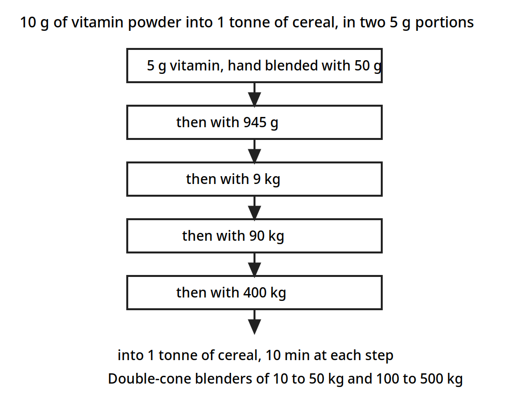
Each 5 g portion is built up step by step so the small part is never less than a tenth of the whole at any step, until it reaches the tonne of cereal.
Diagram for Example 12.3: staged dilution ladder, drawn from the book data.
The rate of mixing follows dM/d theta = K (1 - M), equation 12.5, so 1 - M = e^(-K theta), equation 12.6. The constant K belongs to the machine and the conditions, and it is found by experiment.
Example 12.4: starch and dried vegetable. In a batch mixer blending starch and dried-powdered vegetables for a soup mixture, the initial proportions of dried vegetable to starch are 40 to 60. The variance of the sample compositions, measured in terms of fractional compositions of starch, is 0.0823 after 300 s of mixing. For how much longer should the mixing continue to reach a specified maximum sample composition variance of 0.02? Assume the starch and vegetable particles are of approximately the same physical size and that a sample holds 24 particles.
Taking the fractional content of dried vegetables as p = 0.4, (1 - p) = 0.6, s_0^2 = 0.4 x 0.6 = 0.24, and s_r^2 = s_0^2 / N = 0.24 / 24 = 0.01. The mixing index is (M) = (s_0^2 - s^2) / (s_0^2 - s_r^2) = (0.24 - 0.0823) / (0.24 - 0.01) = 0.685. From equation 12.6, e^(-300 K) = 1 - 0.685 = 0.315, so 300 K = 1.55, and K = 5.2 x 10^-3. For s^2 = 0.02, (M) = (0.24 - 0.02) / (0.24 - 0.01) = 0.957, so 0.957 = 1 - e^(-5.2 x 10^-3 theta), giving theta = 603 s, say 600 s. The additional mixing time would be 600 s - 300 s = 300 s: as much again as has already been spent, to buy the last part of the evenness.
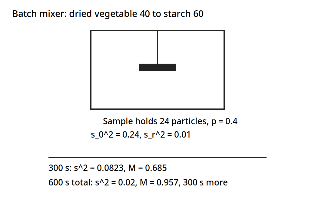
A batch mixer blending starch and dried vegetable, 40 to 60. After 300 s the variance is 0.0823; 300 s more, 600 s in total, brings it to the specified 0.02.
Diagram for Example 12.4: batch mixer, drawn from the book data.
12.7 Energy in mixing: the dough mixer
Quite substantial quantities of energy can be consumed in some types of mixing, such as the mixing of plastic solids. There is no necessary connection between energy consumed and the progress of mixing: shearing along one plane, then recombining to restore the original arrangement, then repeating, would consume energy but accomplish no mixing at all. In well-designed mixers energy input does relate to mixing progress, though the actual relationship has normally to be determined experimentally. In the mixing of flour doughs using high-speed mixers, the energy consumed, or the power input at any particular time, can be used to determine the necessary mixing time, because mixing combines with chemical reaction as the flour oxidizes during mixing, which leads to increasing resistance to shearing and so to increased power being required to operate the mixer.
Example 12.5: a dough mixer. In a particular mixer used for mixing flour doughs for breadmaking, it has been found that mixing can be characterized by the total energy consumed, and that sufficient mixing has been accomplished when 8 watt hours of energy have been consumed by each kg of dough. Such a mixer, handling 2000 kg of dough, is observed just after starting to be consuming 80 amperes per phase, which rises steadily over 10 s to 400 amperes, at which level it then remains effectively constant. The mixer is driven by a 440-volt, 3-phase electric motor with a power factor (cos phi) of 0.89, and the overall mechanical efficiency between motor and mixing blades is 75%. Estimate the necessary mixing time.
Power to the motor is sqrt(3) E I cos phi, where I is the current per phase and E and cos phi are 440 volts and 0.89 respectively. In the first 10 s, I_average = 1/2 (80 + 400) = 240 amperes. The energy consumed in the first 10 s is 130.5 watt hours, which is 130.5 / 2000 = 0.06 Wh/kg. The energy still needed after the first 10 s is (8 - 0.06) = 7.94 Wh/kg. The additional time needed, at steady 400 ampere current, is (7.94 x 2000 x 3600) / (1.73 x 400 x 440 x 0.75 x 0.89) = 281 s. The total time is 281 + 10 = 4.9 min. In actual mixing the power consumed would decrease slowly, by around 10 to 15% over the mixing process.
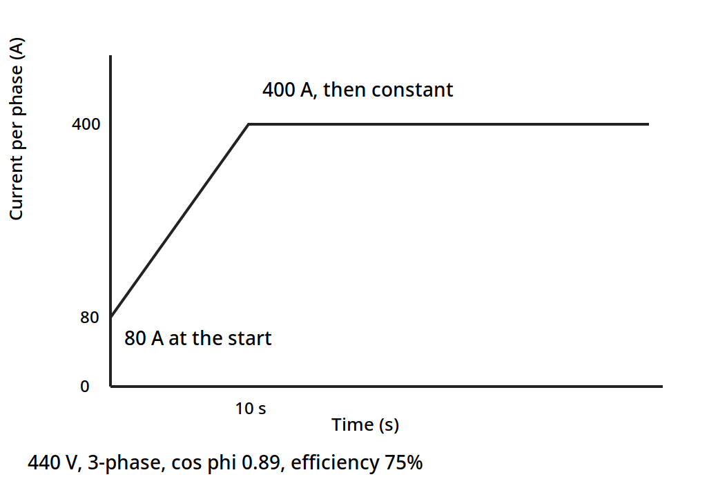
The current rises from 80 A to 400 A in the first 10 s and then stays constant. 8 Wh/kg are needed for 2000 kg of dough: the first 10 s use 130.5 Wh as printed (0.06 Wh/kg), 7.94 Wh/kg are still needed, 281 s more at 400 A, 4.9 min in total.
Diagram for Example 12.5: current against time, drawn from the book data.
One check on the book must be stated plainly. The additional-time line recomputes exactly from the stated current, voltage, power factor and efficiency, giving 281 s. The first-10-seconds line as printed does not: putting I = 240 A, E = 440 V, cos phi = 0.89 and efficiency 0.75 into the stated power formula gives about 339 Wh for 10 s, not the 130.5 Wh the book prints. The book's downstream numbers, 0.06 Wh/kg remaining, 7.94 Wh/kg still needed, 281 s additional and 4.9 min total, all follow from the printed 130.5 Wh, so this unit keeps the book's numbers as printed and flags the discrepancy rather than silently changing any of them.
Quick check
A dough mixer needs 8 Wh per kg, and after 10 s it has used 0.06 Wh per kg. Roughly how much of the job, in energy terms, is still to be done?
Check your answer
Almost all of it: 7.94 of the 8 Wh per kg, about 99%, is still to come. The first 10 seconds barely start the job.
12.8 Liquid mixing: power numbers and scale-up
Food liquid mixtures can be sampled and analysed the same way as solid mixtures, but most of the information available concerns the power requirements for the most commonly used liquid mixer, some form of paddle or propeller stirrer. In these mixers the fluids to be mixed are placed in containers and the stirrer is rotated, and the measurements have been made in terms of dimensionless ratios involving all of the physical factors which influence power consumption. The results are correlated in an equation of the form (Po) = K (Re)^m (Fr)^n, equation 12.7, where (Re) = D^2 N rho / mu, (Po) = P / (D^5 N^3 rho), which is called the Power number, and (Fr) = D N^2 / g, which is called the Froude number. D is the diameter of the propeller, N is the rotational frequency of the propeller in rev/min, rho is the density of the liquid, mu is the viscosity of the liquid, and P is the power consumed by the propeller. The Reynolds number uses the product D N for the velocity, which differs by a factor of pi from the actual velocity at the tip of the propeller.
The Froude number correlates the effects of gravitational forces, and it only becomes important when the liquid surface is disturbed by the propeller. Below Reynolds numbers of about 300 the Froude number is found to have little or no effect, so equation 12.7 becomes (Po) = K (Re)^n, equation 12.8. Experimental results from the work of Rushton are shown plotted in Fig. 12.1. No general formulae have been obtained, so the results are confined to the particular experimental propeller configurations which were used. For a propeller with a pitch equal to the diameter, Rushton gives n = -1 and K = 41. Where experimental results are not already available, the best approach to the prediction of power consumption in propeller mixers is to use physical models, measure the factors, and then use equation 12.7 or equation 12.8 for scaling up the experimental results.
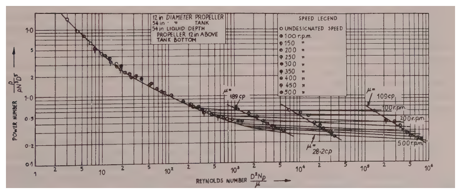
Figure 12.3: Performance of propeller mixers, from Rushton (1950). (Earle, Fig. 12.1, p. 171.) The axes, the box text, the speed legend and the curve pattern follow the book. The chart is a log-log plot of many measured points.
Example 12.6: scaling a propeller mixer up. Vitamin concentrate is being blended into molasses, and satisfactory mixing rates can be obtained in a small tank 0.67 m in diameter with a propeller rotating at 450 rev/min. If a large-scale plant is to be designed which will require a tank 2 m in diameter, what will be suitable values to choose for tank depth, propeller diameter and rotational speed, if it is desired to preserve the same mixing conditions as in the smaller plant? What would be the power requirement for the motor driving the propeller? Assume the viscosity of molasses is 6.6 N s/m2 and its density is 1520 kg/m3.
Use the subscripts S for the small tank and L for the larger one. To preserve geometric similarity the dimensional ratios should be the same in the large tank as in the small. Given that the full-scale tank is three times larger than the model, D_L = 3 D_S, H_L = 3 H_S = 3 x 0.75 = 2.25 m, the depth of the large tank, and the propeller diameter in the large tank is D_L = 3 D_S = 3 x 0.33 = 1 m. For dynamic similarity, (Re)_L = (Re)_S, so D_L^2 N_L = D_S^2 N_S, and N_L = (1/3)^2 x 450 = 50 rev/min = 0.83 rev/sec, the speed of the propeller in the large tank.
Now (Re) = (D_L^2 N_L rho / mu) = (1^2 x 0.83 x 1520) / 6.6 = 191, so equation 12.8 is applicable, and assuming K = 41 and n = -1, (Po) = 41 (Re)^-1 = P / (D^5 N^3 rho), so P = (41 x 1^5 x (0.83)^3 x 1520) / 191 = 186 J/s. A tank three times as wide, turning nine times more slowly, needs only about a quarter of a horsepower to stir the molasses the same way.
12.9 Mixers and baffles: stopping the swirl
An impeller gives the liquid three kinds of flow: radial, longitudinal and rotational. The radial and longitudinal components generally contribute to mixing, but the rotational component may not. An impeller rotating on a vertical shaft mounted centrally in the vessel makes the liquid flow in a circular path around the shaft: the flow is generally laminar, layers form in the liquid, little or no longitudinal flow occurs between the layers, and the vessel contents simply rotate with little mixing. Since the relative velocity between the impeller blade and the liquid is low, the power that can be absorbed by the liquid is limited. The tangential component can also form a vortex at the surface, which deepens as the speed rises; once the vortex reaches the suction of the impeller the power imparted to the liquid is suddenly reduced and air is drawn in. Solid particles may also separate out under centrifugal force.
Vortexing is reduced by positioning the agitator off-centre, or by baffles: vertical strips fixed perpendicular to the wall of the vessel, four of which are generally sufficient. Baffles interrupt the rotational flow and turn it into the radial and longitudinal flow that mixes.
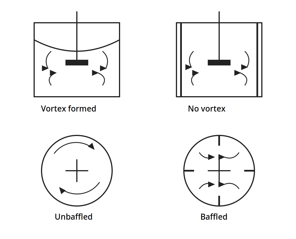
Top: side views. Without baffles the surface dips into a deep vortex; with baffles the surface stays flat and the flow circulates. Bottom: plan views. Without baffles the liquid goes around in a circle; with four baffles it is thrown outward and mixed.
Figure 12.4: Flow patterns in baffled and unbaffled vessels with paddle or turbine agitators. (Brennan, Fig. 5.1, p. 69.)
The agitators themselves are chosen by the job. Paddle agitators run at 20 to 150 rev/min, with blades about one fifth as wide as they are long. Turbine agitators run at 30 to 500 rev/min, at 30 to 50% of the vessel diameter. Propeller agitators run at 500 to several thousand rev/min, at less than one third of the vessel diameter. Vessels are usually vertical cylindrical tanks with dished bottoms, filled so the liquid depth to vessel diameter ratio is usually 0.5 to 1.5, with 1.0 recommended, and one impeller per vessel diameter of height.
Dry solids mix by three mechanisms: convection, the bulk movement of groups of particles; diffusion, the random movement of single particles; and shear, the slipping of layers over one another. They also segregate, by size, shape and density, which is why a mixture that was even can become patchy again. Tumbler mixers, such as double-cone and ribbon mixers, run at 50 to 60% working capacity and up to 100 rev/min. Ribbon mixers and vertical screw mixers suit powders, and fluidized-bed mixers suit free-flowing solids. Pan mixers with planetary motion and trough kneaders with Z-blade or sigma blades suit pastes and doughs. Gould's mixing chapter adds the plant view: jacketed kettles and process tanks, batch and continuous systems, and the same staged care with small additions.
12.10 Emulsification: keeping two liquids together
An emulsion is one liquid dispersed as droplets in another liquid that it does not mix with. Milk is fat in water, butter is water in fat, mayonnaise is fat in water, and ice cream is fat in water, then frozen. The droplets are commonly 1 to 10 micrometre across, and below 0.1 micrometre they are colloidal. Stability follows Stokes law: a droplet rises or falls at v = D^2 g (rho_p - rho_f) / (18 mu), so smaller droplets and a more viscous continuous phase both slow the separation. Homogenizing milk breaks the fat globules small enough that cream stops rising in the bottle.
Emulsifying agents sit at the interface and keep the droplets apart. Brennan lists proteins, phospholipids, sterols, glycerol esters, propylene glycol esters, sorbitan esters, cellulose ethers, carboxymethyl cellulose, bentonite, carbon black, and soaps such as sodium palmitate, whose molecules orient at the interface with one end in the water and one end in the oil. A phase volume ratio above 50% is difficult to hold, because the droplets crowd each other. Temperature matters: up to 160 F for milk products, and lower for egg yolk products, which are heat sensitive.
The machines that make emulsions all break droplets by force. Pressure homogenizers force the liquid through a valve gap a few thousandths of an inch wide at up to 10,000 psi, with velocities of 950 ft/sec reported, giving droplets of 0.1 to 0.2 micrometre, and as low as 0.02 micrometre. A second-stage valve at 400 to 500 psi breaks up clusters, and milk fat globules come out at 1 to 2 micrometre. Earle puts the homogenizer pressures of the order of 7 x 10^3 kPa. Colloid mills pass the liquid through a clearance of 0.002 to 0.05 inch between a rotor and a stator, at 3000 rev/min for a 15 inch rotor to 15,000 rev/min for a 3.5 inch rotor, giving droplets of 1 to 2 micrometre: better than homogenizers above 1000 cP, while homogenizers are better below 200 cP. Ultrasonic homogenizers use a wedge resonator at 18 to 30 kHz with a feed at 50 to 200 psi, giving droplets of 1 to 2 micrometre.
Buttermaking is emulsification in reverse. Cream at 35 to 40% fat is chilled and aged, then churned: the fat globules are broken, the fat comes together, and the emulsion inverts from oil-in-water to water-in-oil, which is butter. The working that follows squeezes out the buttermilk and spreads the remaining water into fine droplets. Continuous methods use the Fritz principle, or a concentrated cream of about 80% fat. Margarine is a water-in-oil emulsion made the other way around, in scraped-surface heat exchangers called votators, which cool the emulsion while scraping it from the wall so it sets evenly.
Quick check
Mayonnaise is fat droplets in water, and butter is water droplets in fat. What is the name for the change from one to the other during churning?
Check your answer
Phase inversion: the emulsion turns inside out, from oil-in-water to water-in-oil.
12.11 What the books do and do not give
Ibarz has no size reduction or mixing chapter, so this unit leans on Earle Chapters 11 and 12 and Brennan Chapters 4 and 5, with Ibarz Chapter 6 rheology only as supporting theory for mixing, as the outline says. Gould Chapters 6, 7 and 12 give the plant practice of disintegration and mixing, with almost no calculations, and they are used here for equipment pictures and plant flow only. Earle gives the worked examples in this unit, 11.1, 11.2, 12.1, 12.2, 12.3, 12.4, 12.5 and 12.6, with the numbers checked twice against the page images, except for the one discrepancy in Example 12.5, which is flagged in section 12.7 rather than hidden. The outline lists Ibarz Problems for this unit, and the book's end-of-chapter problems for Chapter 6 are rheology problems, not mixing design problems, so no Ibarz problem is presented here as a mixing worked example.
Try it yourself: Put a spoonful of oil and a spoonful of water in a small jar and shake it hard. Watch the cloudy mixture clear as the droplets join and rise: that is an emulsion without an emulsifying agent, and it does not last. Now add a drop of dish soap, which is an emulsifying agent like the ones in section 12.10, and shake again: the cloud lasts far longer, and the droplets stay small. Then take a tub of cream and whisk it past the whipped stage: it turns grainy, then yellow, then buttery, and liquid separates out. That is phase inversion, the churning of section 12.10, in a bowl.
Key ideas to carry forward
- Size reduction opens surface so later steps work faster, and the reduction ratio runs below 8 to 1 for coarse crushers and up to 100 to 1 for fine grinding.
- Kick's law fits coarse grinding, Rittinger's law fits fine powders, and Bond's law sits between them with the work index E_i.
- Bond's law says a 5 hp motor grinding sugar to 88 micrometre would need 5.4 hp to grind to 125 micrometre at 50% more throughput, so the motor is not enough.
- Surface area per unit mass grows as particles get smaller: 5% of a salt sample in a fine fraction carries 16.6 m2 of surface against 7.88 m2 for 38% in a coarse fraction.
- A ball mill runs best at about 75% of its critical speed, N_c = 76.6 / sqrt(2R).
- Honey is nearly Newtonian with n = 0.989, while ketchup, mayonnaise and peanut butter are strongly pseudoplastic, with n from 0.065 to 0.196.
- Mixing is measured by the variance of samples, and the mixing index M runs from 0 for unmixed to 1 for randomly mixed.
- A dough reaches M = 0.93 in 5 minutes and 0.99 in 10 minutes: the last part of evenness costs the most time.
- A tiny addition needs staged dilution: 10 g of vitamin powder into a tonne of cereal is built up through steps where it is never less than 10% of the mixture.
- In Example 12.4, starch and vegetable need 600 s in total to reach a variance of 0.02, which is 300 s more than the 300 s already spent.
- A dough mixer needing 8 Wh per kg takes 4.9 minutes for 2000 kg of dough, and the book's first-10-seconds line of 130.5 Wh does not recompute from its own stated current and voltage, so it is flagged, not hidden.
- A propeller mixer scales by keeping the Reynolds number the same: a tank three times as wide needs a propeller three times as wide turning nine times more slowly, and the molasses plant of Example 12.6 needs 186 J/s.
- Baffles turn the useless rotational flow in a tank into the radial and longitudinal flow that mixes, and stop the vortex that draws air in.
- Homogenizers make droplets of 0.1 to 0.2 micrometre at up to 10,000 psi, and churning inverts cream from oil-in-water to water-in-oil to make butter.
Glossary
Size reduction
Making solid pieces smaller by crushing, impact or shear. Food tech example: grinding wheat kernels into flour in a hammer mill.
Reduction ratio
The average size of the feed over the average size of the product. Food tech example: a coarse crusher working at a ratio below 8 to 1.
Kick's law
The grinding law that energy is proportional to the size reduction ratio, fitting coarse grinding. Food tech example: crushing a material from 10 cm to 5 cm for the same energy as from 5 mm to 2.5 mm.
Rittinger's law
The grinding law that energy is proportional to the new surface created, fitting fine powders. Food tech example: the extra energy needed to grind a fine flour, where the new surface is large.
Bond's law
The intermediate grinding law using the work index E_i, the energy to reduce unit mass to 80% passing 100 micrometre. Food tech example: the sugar grinding calculation of Example 11.1.
Work index
The energy needed to reduce unit mass of a material from an infinitely large size to 100 micrometre, in Bond's law. Food tech example: the E_i that fixes the sugar grinding power in Example 11.1.
Shape factor
A number, lambda, that relates a particle's surface to its size, about 1.75 for ground materials and 1 for a cube or a sphere. Food tech example: the 1.75 used for ground salt in Example 11.2.
Specific surface
The surface area per unit mass of a powder. Food tech example: a fine flour with a large specific surface that oxidizes faster than whole grain.
Hammer mill
A mill in which swinging hammers on a fast rotor break material against a casing until it passes a screen. Food tech example: grinding spice or grain to a fine powder.
Ball mill
A rotating cylinder in which tumbling balls grind the material. Food tech example: fine grinding run at about 75% of the critical speed.
Critical speed
The speed at which the balls in a ball mill centrifuge to the wall and stop grinding. Food tech example: N_c = 76.6 / sqrt(2R) rev/min.
Screening
Sorting particles by size on meshes, with the undersize passing and the oversize held back. Food tech example: a Tyler sieve series separating ground salt into fractions.
Rheology
The study of how materials flow and deform. Food tech example: the power law parameters for ketchup and honey in Table 12.2.
Newtonian liquid
A liquid whose viscosity does not change with the rate of shear. Food tech example: honey, with a flow index n of 0.989.
Pseudoplastic
A liquid whose apparent viscosity falls as the shear rate rises, flowing more easily once it is moving. Food tech example: ketchup, with a flow index n of 0.136.
Viscoelastic
A material showing the properties of a viscous liquid and an elastic solid together. Food tech example: a dough that flows under a roller and springs back when the roller lifts.
Mixing index
A number from 0 to 1 that says how mixed a mixture is, from the variance of samples. Food tech example: a dough at M = 0.93 after 5 minutes of mixing.
Variance
A measure of how much sample compositions differ from their mean, used to judge how even a mixture is. Food tech example: s^2 = 1.51 x 10^-7 for the salt and magnesium carbonate mixture.
Staged dilution
Building a tiny addition up through a series of larger mixtures so it spreads evenly. Food tech example: 5 g of vitamin powder blended into 50 g, then 945 g, then 9 kg, then 90 kg, then 400 kg of cereal.
Baffle
A vertical strip fixed to the wall of a mixing vessel to break up rotational flow and stop vortexing. Food tech example: four baffles in a tank holding a paddle agitator.
Vortex
A dip in the surface of a stirred liquid, caused by rotational flow, which can draw air into the mixture. Food tech example: the deep vortex in an unbaffled tank in Figure 12.4.
Power number
A dimensionless number, P / (D^5 N^3 rho), used to predict the power of a propeller mixer. Food tech example: the power number curve for Rushton propellers in Figure 12.3.
Emulsion
One liquid dispersed as droplets in another liquid that it does not mix with. Food tech example: mayonnaise, with fat droplets in water.
Emulsifying agent
A substance that sits at the interface between two liquids and keeps the droplets from joining. Food tech example: egg yolk lecithin holding mayonnaise together.
Homogenizer
A machine that forces a liquid through a narrow valve gap at high pressure to break droplets very small. Food tech example: a homogenizer making milk fat globules 1 to 2 micrometre across so cream stops rising.
Phase inversion
An emulsion turning inside out, so the liquid that was the droplets becomes the continuous phase. Food tech example: cream churning from oil-in-water to water-in-oil to make butter.
References
- Earle, R. L., Unit Operations in Food Processing, 2nd edition, Pergamon Press, 1983. Chapter 11, Size Reduction, including Figures 11.1 and 11.2 and Examples 11.1 and 11.2; Chapter 12, Mixing, including Figure 12.1 and Examples 12.1 to 12.6.
- Brennan, J. G., Butters, J. R., Cowell, N. D., and Lilly, A. E. V., Food Engineering Operations, Elsevier, 1969. Chapter 4, Size Reduction and Screening of Solids, including Figure 4.3; Chapter 5, Mixing and Emulsification, including Figure 5.1.
- Ibarz, A., and Barbosa-Canovas, G. V., Unit Operations in Food Engineering, CRC Press, 2003. Chapter 6, Rheology of Food Products, including Tables 6.1 and 6.3, as supporting theory for mixing.
- Gould, W. A., Unit Operations for the Food Industries, CTI Publications, 1996. Chapter 6, Disintegration, Little Change in Form; Chapter 7, Disintegration, Considerable Change in Form; Chapter 12, Mixing and Blending.
- Kokini, J. L., Rheological properties of foods, in Handbook of Food Engineering, Heldman, D. R., and Lund, D. B., Eds., Marcel Dekker, New York, 1992, as cited in Ibarz, Chapter 6, for Table 6.3.
- Muller, H. G., An Introduction to Food Rheology, Crane, Russak and Co., New York, 1973, as cited in Ibarz, Chapter 6, for Table 6.1.
- Rushton, J. H., 1950, as cited in Earle, Chapter 12, for Figure 12.1.